Introduction

Variation and change are pervasive in the natural world. Ecosystem processes and the resulting ecosystem attributes are dynamic and complex due to multiple factors affecting them (Southwood, 1995; Sinclair & Byrom, 2006; Butler & O’Dwyer, 2020). Examples of the most widely studied ecosystem processes are those related to biogeochemical cycles, climate change, primary productivity, and disturbance and ecological succession (Bennett et al., 2009; Harrison et al., 2014; Poorter et al., 2023). The large variability of these processes in all ecosystems worldwide has fostered the development of many methods for their study, as choosing a particular method largely depends on the specific attributes of each system and study goals.

During the last half century, ecosystem science has greatly benefited from the development of remote sensing (Turner et al., 2003; Kuenzer et al., 2011; Wang et al., 2012; Pettorelli et al., 2014). This development has accelerated the emergence and diversification of new approaches to studying vegetation, which is the most conspicuous ecosystem component and, given the comparatively great longevity of plants, particularly of woody species, and their sessility, perhaps the one showing the slowest changes (Mezaal et al., 2017; Einzmann et al., 2021; Ibarra-Manríquez et al., 2022). A major contribution of remote sensing to ecosystem studies has been through the construction of mathematical models aimed at describing, estimating, and predicting ecosystem attributes (e.g., Aschbacher et al., 1995; Ramsey III & Jensen, 1995; Kayitakire et al., 2006; Proisy et al., 2007; Fatoyinbo & Armstrong, 2010; Gallardo-Cruz et al., 2012). Mathematical models are instrumental in explaining ecosystem variability (Hillier & Lieberman, 1990; Cavender-Bares et al., 2022) as they establish quantitative relationships between ecosystem or vegetation properties and a set of external variables provided by remote sensing. Inverse modeling, an alternative process that involves the use of observed data to infer parameters or conditions that best fit the models and allows predicting ecosystem attributes in sites lacking field data (Zhang et al., 2024), is also key to advancing our knowledge of ecosystem dynamics.

Here, we provide an overview of the potential of remote sensing to support efforts of ecosystem attribute modeling, particularly of its plant community component. Our objectives were: (i) to review concepts of vegetation structure and structural complexity, (ii) to summarize advantages and shortcomings of remote sensing inputs and modeling approaches, and (iii) to contrast the empirical vs. physical modeling, and to introduce the hybrid modeling approach based on the combination of these two main approaches. Because empirical and physical modelling currently represent the two most widely used approaches in remote sensing-based vegetation studies, our review excludes other perspectives such as data fusion (Zhang, 2010; García et al., 2018).

Vegetation structure and structural complexity

Almost three-quarters of a century ago, Dansereau (1957) defined vegetation structure as the spatial organization of individuals that constitute a plant community. While spatial organization is undoubtedly a fundamental property of plant communities (Terradas, 2001), it is not the sole structural component. In a broader sense, vegetation structure refers to how these components (i.e., plants) are organized in the three-dimensional space and is primarily defined by their physical and quantitative structure (Kershaw & Looney, 1985; Norman & Campbell, 1989; Meave & Pérez-García, 2013). The physical structure is expressed in two dimensions: the vertical arrangement of plants or their parts, i.e., the distribution of community components along the vertical axis (community’s vertical stratification or vertical differentiation), and the horizontal arrangement, which refers to how the components are distributed across the terrain occupied by the community (spatial distribution of species and individuals; Popma et al., 1988; Campbell & Norman, 1989; Bongers, 2001). The quantitative structure relates to the use of numeric variables to evaluate community properties, such as species abundance or basal area (Morin, 1999; Magurran, 2004). Though ideally the study of plant community structure should encompass all its components, including all of them in individual studies is uncommon (Crawley, 1997). The structural component has been the most extensively addressed in vegetation research, particularly in terms of density of individuals or the biomass contributed by each species to the community (quantitative or taxonomic structure; Barbosa et al., 2014; Dube et al., 2016; Zhang et al., 2019). However, significant emphasis has also been placed on quantifying species composition (floristic structure; Mueller-Dombois & Ellenberg, 1974; Kent, 2012).

Related to the concept of community structure is that of structural complexity. Though similar, these two concepts refer to different community attributes. Community structural complexity is more closely related to the variability of its structural components (Cadenasso et al., 2003; LaRue et al., 2019; Lian et al., 2022). Accordingly, a complex community exhibits substantial variation in several dimensions, including biomass, plant height, canopy openness, and their concentration or dispersion in space (McCoy & Bell, 1991). Also, more complex communities tend to host a larger number of species with the concomitant greater diversity of growth forms, crown shapes, trunk diameters (in the case of forest communities), branching patterns, leaf sizes and various functions related to water and carbon economies (Huston, 1994; Bongers, 2001; Mejía-Domínguez et al., 2011; van der Sande et al., 2024). Although one could naturally assume that forests are more complex than non-forest communities, there are examples of the stringing complexity of non-forest vegetation (e.g., Valiente-Banuet et al., 2000).

In addition to the variation of vegetation community attributes through space, these can also be heterogeneous along the temporal dimension. Succession is the ecological process that best allows the observation of changes in vegetation complexity over time (Connell & Slatyer, 1977; Poorter et al., 2024). Through succession, vegetation complexity increases regarding the variability of the physical, taxonomic and floristic structure of the community (Lebrija-Trejos et al., 2011; Anyomi et al., 2022; Poorter et al., 2023).

Remote sensing has transformed the monitoring of biological diversity through structural, compositional, and functional measurements of ecosystems (Turner et al., 2003; Pettorelli et al., 2014; Dube et al., 2016; Cavender-Bares et al., 2022). The use of remote sensing takes advantage of the inherent natural variability of plant communities with different complexity to study them through structural and compositional data (Dronova & Taddeo, 2022), and aims to describe ecosystem states, monitor them over time, and utilize the significance of these variables to build models capable of predicting or estimating structural attributes (Asner et al., 2003; Gallardo-Cruz et al., 2012; Fassnacht et al., 2024). For example, studies of ecological succession can greatly benefit from the use of remote sensing inputs, like LiDAR to assess canopy height development (García et al., 2018), or multispectral imagery to examine phenological patterns using vegetation indices (Manzo-Delgado & Meave, 2003).

Remote sensing in ecosystem and vegetation studies

Since the early second half of the 20th century remote sensing has been an attractive alternative for studying all ecosystems of the planet (Turner et al., 2003; Aplin, 2004; Chuvieco, 2016; Ibarra-Manríquez et al., 2022). At present, most research in this field of study is based on the use of satellite imagery; however, this is by no means the only remote sensing input used in the past or the present to study plant communities (Chinea, 2002; Navulur, 2007; Anderson & Gaston, 2013; Feldman, 2024). For example, aerial photography was widely used prior to the great diversification of sensors mounted on satellite platforms and it is still used in analysis of historical trends of ecosystem changes (Morgan et al., 2010; Chávez et al., 2024). The comparison of aerial photography, satellite imagery, and more recently, UAV (unmanned aerial vehicle) imagery reveals fundamental differences among these remote sensing inputs used in vegetation studies (Feng et al., 2015; Eide et al., 2021; Alvarez-Vanhard et al., 2021; Li et al., 2023). UAV imagery, though capable of greater detail and increasing accessibility, is constrained by its limited coverage area for data acquisition. Conversely, air photographs, but particularly satellite imagery, offer the possibility to cover much larger areas, with different spatial resolutions. In turn, not all satellite imagery is freely available to every user, and despite their prominent role in vegetation monitoring and mapping studies at present (Wulder et al., 2022; Chávez et al., 2024), it is noteworthy that aerial photography continues to be part of the remote sensing arena, particularly for precise cartography often linked to forestry (Fleming et al., 2025), and time series reconstruction covering periods predating satellite imagery (Fernández-Pacheco et al., 2023). Although there are different types of remote sensors (e.g., SAR, LiDAR, multispectral, hyperspectral), the following sections will focus mainly on multispectral and hyperspectral.

The physics of the spectral remote sensing

In remote sensing studies based on satellite imagery, all sensors that gather digital information from satellite platforms lie on the same physical principles (Navulur, 2007; Schott, 2007; Knudby, 2021). These principles involve capturing electromagnetic signals reflected by surfaces for the interpretation of the elements present on the terrain, as each material reflects light in a specific way according to its physical and structural properties (Tippens, 2011). Each object has a spectral signature based on how it reflects and emits electromagnetic radiation (Turner et al., 2003; Schowengerdt, 2007). Particularly, in plant community studies, plant reflectance is used in the wavelengths corresponding to the visible portion of the electromagnetic spectrum (red, green, and blue bands), as well as the near and far-infrared regions (Jensen, 2007; Lillesand et al., 2015; Li et al., 2023).

The absorption limit of chlorophyll is in two regions; solar light is strongly absorbed in the blue (490 nm) and red (676 nm) regions, while the green light (554 nm) is little or not absorbed at all, depending on the photosynthetic pigment. In the light received by plants a region known as the red edge, located around 700 nm, is fundamental for remote sensing because this region constitutes an abrupt limit between absorption and reflectance in plants (Delegido et al., 2011; Peña et al., 2019; Zhang et al., 2022; Fig. 1). The red edge results from two special optical properties of plant tissues: there is high absorption by chlorophyll in the visible red region, but as the wavelengths slightly increase, reflectance increases rapidly in the near-infrared (Smith et al., 2004; Jones & Vaughan, 2010). This feature has a very important physiological basis: by reflecting the energy at this latter wavelength, plants avoid overheating and the consequent permanent physiological damage. The existence of the red edge provides the basis for vegetation identification and assessment procedures using combinations of red and infrared radiation through indices that will be discussed later (Horler et al., 1983; Bramich et al., 2021).

Like any surface, plants’ spectral characteristics can be captured by remote sensors mounted on satellites. Thus, it is possible to establish relationships between the biophysical characteristics of the terrain, and two attributes present in all satellite images: image tone and image texture (Haralick et al., 1973; Haralick, 1979; Strahler et al., 1986; Woodcock & Strahler, 1987). Tone is defined as the mean spectral value captured by the sensor in each pixel and is associated with a reflectance value. Reflectance, in turn, refers to the amount of light reflected per unit area at a specific site (Chinea, 2002). Unlike tone, image texture refers to the spatial arrangement of its pixels and the differences between them in each scene (Haralick, 1979). The use of these variables in vegetation studies has been important to understanding the characteristics of the ecological system studied (Haralick, 1979; Strahler et al., 1986; Shaw & Burke, 2003). Notably, most studies have focused on image tone to analyze the radiometric properties of plant communities (e.g., Schlerf et al., 2005; Ustin & Gamon, 2010; Zhang et al., 2014; Rossi et al., 2021; Feldman, 2024; Kötz et al., 2024), while studies focused on the analysis of texture are still scant but rapidly increasing (e.g., Feng et al., 2015; X. Wang et al., 2023; Du et al., 2024).

Absorption spectra of chlorophyll a and chlorophyll b in plant tissues. Chlorophyll a (green curve) has absorbance peaks around 430 nm and 665 nm, while chlorophyll b (purple curve) absorbs more efficiently around 455 nm and 640 nm. In remote sensing studies, the sharp transition from high absorbance to high reflectance between the red and near-infrared regions, known as the red edge (approximately around 700 nm and illustrated here as a red bar), was used to construct various vegetation indices relating the reflectance in these regions that provide indicators of photosynthetic activity and vegetation health

Figure 1. Absorption spectra of chlorophyll a and chlorophyll b in plant tissues. Chlorophyll a (green curve) has absorbance peaks around 430 nm and 665 nm, while chlorophyll b (purple curve) absorbs more efficiently around 455 nm and 640 nm. In remote sensing studies, the sharp transition from high absorbance to high reflectance between the red and near-infrared regions, known as the red edge (approximately around 700 nm and illustrated here as a red bar), was used to construct various vegetation indices relating the reflectance in these regions that provide indicators of photosynthetic activity and vegetation health.

Figura 1. Espectros de absorción de la clorofila a y la clorofila b en tejidos vegetales. La clorofila a (curva verde) presenta picos de absorción alrededor de 430 nm y 665 nm, mientras que la clorofila b (curva morada) absorbe con mayor eficiencia en torno a 455 nm y 640 nm. La transición abrupta de alta absorbancia a alta reflectancia entre el rojo y el infrarrojo cercano, conocida como la pared roja (aproximadamente a los 700 nm e ilustrada aquí como una barra roja), se usó para construir varios índices de vegetación que relacionan la reflectancia en estas regiones y que sirven de indicadores de la actividad fotosintética y la salud de la vegetación.

Resolution of remote sensing inputs

In remote sensing-based vegetation studies, extracting information from satellite imagery hinges on selecting appropriate variables and scales (Woodcock & Strahler, 1987; Guan et al., 2012; Obata et al., 2012; Steenvoorden et al., 2023). Satellite images are characterized by two types of resolution, namely spatial and spectral resolution. In addition, the frequency with which these images are acquired defines their temporal resolution. The three types of resolution, which can be conceived as a spatial-spectral-temporal resolution complex of remote sensing imagery (Q. Wang et al., 2023), are key for interpreting remote sensing data, enabling sensors to capture terrain features ranging from centimeters to thousands of meters, spectral information across various wavelengths (Singh, 1989; Navulur, 2007; Schowengerdt, 2007; Nagendra & Rocchini, 2008), and ecological processes occurring over different time periods (Willis, 2015).

Spatial resolution is the smallest discernible visualization of an object in an image (Atkinson & Aplin, 2004) and allows appreciating the variation of the objects contained in it (Strahler et al., 1986; Foody & Cutler 2001; Nagendra & Rocchini, 2008; Wang et al., 2010). Pixels are squared units of an image containing a fraction of the radiometric information reflected by the surface and their size determines their capacity to detect the details of the spatial elements on the terrain (Atkinson & Aplin, 2004; Leduc & Knudby, 2018; Lyu et al., 2022). Pixel size defines such level of detail and varies depending on the sensors’ detection capabilities. Navulur (2007) proposed four resolution categories according to pixel size: (i) low resolution, with pixels > 30 m; (ii) medium resolution, > 2 to ≤ 30 m; (iii) high resolution, 0.5 - 2 m; and (iv) very high resolution, < 0.5 m. Although remote sensing studies have used images of all four resolution categories, high and very high spatial resolutions are commonly used in current environmental research because they increase precision in identifying and characterizing small objects on the ground (Nagendra & Rocchini, 2008; Wolter et al., 2009; Wang et al., 2010; Myint et al., 2011; Morin et al., 2019; Ahmad et al., 2021). For example, the larger the area to be studied, the lower the spatial resolution tends to be. Similarly, band width in the electromagnetic spectrum captured by a sensor determines its ability to detect spectral differences and constitutes the spectral resolution of the images, which leads to their classification as multispectral or hyperspectral. In turn, temporal resolution refers to the frequency of observations of the same event over time in the same area (Navulur, 2007; Schowengerdt, 2007). These events can be short-lived (such as fires or hurricanes) or processes that require annual assessments (e.g., successional changes in vegetation cover, urban growth, etc.). Although temporal resolution is not a property of the images themselves, it is directly related to the different interpretations of ecological processes recorded in the images. When vegetation monitoring is planned to be conducted over long time periods, it is important to decide the most adequate temporal resolution. For example, the study of a long-term successional process may only require one or a few images per year, whereas the analysis of the leaf flushing periods in a deciduous community could need daily images to capture the detailed dynamics of this process.

An important issue in selecting the most appropriate resolutions (i.e., spatial, spectral, and temporal) for a given study is the existence of trade-offs among these resolutions, which explains why there is no perfect high-resolution sensor in all its components (Fig. 2). The trade-off between spatial and spectral resolution is particularly critical. For example, hyperspectral images provide a very high level of detail in spectral information, with over one hundred continuous spectral bands (Shaw & Burke, 2003; Xie et al., 2008) and thus can be used for highly specific purposes, such as determining the spectral signature of species present in an ecosystem (Blasco et al., 1998; Hossain & Lin, 2003; Adam et al., 2009); however, they lack the ability to capture finer elements in the landscape. By contrast, multispectral images are composed of up to twelve spectral bands, which means that they only contain specific regions of the electromagnetic spectrum (Asner & Heidebrecht, 2002; Adam et al., 2009), but their spatial resolution is higher, better able to capture more detailed elements on the ground (Fig. 2).

Flowchart for guiding the selection of remote sensing imagery based on spatial scale, required precision, the need for temporal monitoring, and spectral resolution. Different levels of spatial and spectral resolution must be considered to optimize information analysis according to the study objectives. The ranges of areas corresponding to the local and regional scales are based on Turner & Gardner (2015). High precision refers to the degree of detail required in the study. Large scale monitoring refers to a large areal coverage of the study.

Figure 2. Flowchart for guiding the selection of remote sensing imagery based on spatial scale, required precision, the need for temporal monitoring, and spectral resolution. Different levels of spatial and spectral resolution must be considered to optimize information analysis according to the study objectives. The ranges of areas corresponding to the local and regional scales are based on Turner & Gardner (2015). High precision refers to the degree of detail required in the study. Large scale monitoring refers to a large areal coverage of the study.

Figura 2. Diagrama de flujo para guiar la selección de imágenes de teledetección en función de la escala espacial, la precisión requerida, la necesidad de monitoreo temporal y la resolución espectral. Se deben considerar distintos niveles de resolución espacial y espectral para optimizar el análisis de la información según los objetivos del estudio. Los intervalos de las áreas que corresponden a las escalas local y regional se basan en Turner y Gardner (2015). El término alta precisión se refiere al grado de detalle requerido en el estudio. Monitoreo de gran escala se refiere a una cobertura grande del área de estudio.

One dilemma faced by vegetation studies using classical remote sensing is the selection of inputs for analysis. Ideally, their spatial and spectral resolutions, along with the temporal resolution of the study, should match the particularities of the studied phenomenon. For one, the best spatial resolution is one that precisely matches the size of the study object (Strahler et al., 1986; Woodcock & Strahler, 1987; Nagendra & Rocchini, 2008); for example, in studying a highly complex plant community, using a very high spatial resolution may be advisable, so that the heterogeneity observed in the image pixels can be explained by the heterogeneity of the plant community components. By contrast, if the spatial resolution is considerably higher than the objects being studied, most measurements in the image will be strongly autocorrelated, and the measurement of local variance will decrease (Strahler et al., 1986; Woodcock & Strahler, 1987). In turn, if the study focuses on a community composed by a large number of species, hyperspectral images are recommended because they can effectively capture the variation in their radiometric signals (Kothari & Schweiger, 2022; Zahra et al., 2024). Therefore, depending on the community attribute being assessed, different types of satellite images can be used.

The influence of instantaneous conditions during image capture

An inherent challenge in studying phenomena on the Earth’s surface from a distance is the interference that occurs during the capture of spectral data in a satellite image (Adjovu et al., 2023; Fichot et al., 2023). Generally, image quality is affected by the interference derived from the physical characteristics of the atmosphere and the surface at the moment of its capture. The behavior of light waves is highly variable, and there are factors that directly or indirectly interfere with the scattering, absorption, and reflection of signals (Tippens, 2011).

The first difficulty faced by remote sensors mounted on satellite platforms is the large distance for detecting radiometric signals. The Earth’s atmosphere reduces the amount of electromagnetic energy reaching the sensor as it disperses and absorbs part of the original signal (Myneni et al., 1995; Chinea, 2002; Chuvieco, 2016). However, the atmosphere is not the only source of interference. Other factors, such as local topography, can create deformations in the image or cast shadows that modify radiometric signal values. The angle of the sun relative to the zenith and the sensor’s viewing angle are also closely related (Singh, 1989; Shepherd & Dymond, 2003; Yin et al., 2022). Spectral values vary depending on the time of image acquisition: capturing an image when the sensor or the sun is at the zenith is different from doing so when either one has a degree of inclination, potentially resulting in the recording of different spectral values (Shaw & Burke, 2003). Despite the development of sun-synchronic sensors that control the relationship between the angle at which the sun illuminates the scene and the angle with which the sensor records the image (Shepherd & Dymond, 2003; Wei et al., 2011), these remain major obstacles that typically arise at the moment of capturing the image. Moreover, in the case of topography, it is impossible to have control over it (Dozier et al., 2022).

Fortunately, at present there are procedures available that correct or minimize these effects, including radiometric, topographic, and atmospheric corrections. The topographic correction does not allow correcting topographic shadows; instead, it focuses on adjusting the image’s geometry to align it correctly with the Earth’s surface (Shepherd & Dymond, 2003; Yin et al., 2022). In turn, the radiometric and atmospheric corrections enable the transformation of reflectance values to physical units at various levels (Wulder et al., 2019; Dozier et al., 2022). Together, these actions make up the image pre-processing phase, which is intended to make the images more suitable for extracting information related to variables that describe the surface (Navulur, 2007).

Remote sensing indices

The tone of the pixels contained in digital images can be used in plant community studies through its incorporation in algorithms known as spectral indices, which relate the electromagnetic energy reflected by the vegetation (and its physical conditions) with the energy detected by remote sensors. Indices are arithmetic combinations of the band channels of an image (Camps-Valls et al., 2012) and their construction is based on the relationships between these bands, which allows for a better assessment of biophysical phenomena in the field. The motivation for the construction of these indices was the need to deal with the interference of physical factors such as soil reflectance, solar illumination, atmospheric conditions, and sensor viewing geometry in detecting spectral values of objects on a given surface with remote sensors (Jensen, 1983; Camps-Valls et al., 2012).

Based on plants’ spectral characteristics, specialized indices have been constructed to study vegetation (Navulur, 2007; West et al., 2019; Zhang et al., 2022; Ståhl et al., 2024). Most vegetation indices currently used can differentiate vegetation from other cover types. This is achieved thanks to the pigments contained in the leaves of plants, in addition to the detection of spectral signatures characteristic of each cover type (Iqbal et al., 2021). The Normalized Difference Vegetation Index (NDVI) and the Enhanced Vegetation Index (EVI) are among the most widely used indices for vegetation monitoring and assessment (Tucker et al., 1985; Gao, 1996; Huete et al., 1997; Blasco et al., 1998; Wang et al., 2010), as they can provide relevant information about its condition at a given time, or to predict attributes such as biomass, structure, and species richness. The design of these indices took advantage of the specific reflectance and absorbance properties of plant pigments (Sinclair et al., 1973; Tucker & Sellers, 1986; Hosgood et al., 1994). The main difference between NDVI and EVI is that the latter reduces the saturation of canopy variations under high photosynthetic activity, thus remaining sensitive to canopy variations, while NDVI does present saturation (Huete, 1988; Huete et al., 1997; Vogelmann et al., 1993). In turn, the Soil-Adjusted Vegetation Index (SAVI) incorporates an adjusted soil constant to minimize the effect of bare soil reflectance in the scene (Huete, 1988), making it a more refined or better-calibrated index. The Normalized Difference Water Index (NDWI) provides a consistent framework for analyzing vegetation health regardless of variations in sensor and illumination conditions while distinguishing water bodies from vegetation and soil (Gao, 1996).

With the development of new sensors with higher spectral resolution (e.g., Sentinel-2), novel indices have been developed to take advantage of these new capabilities, such as indices including the red-edge and narrow NIR (e.g., NDVIre1 (Gitelson & Merzlyak, 1994), NDVIre2, NDVIre1n, and NDVIre2n (Fernández-Manso, 2016), Plant Senescence Reflectance Index (PSRI; Merzlyak et al., 1999); Chlorophyll Index Red-edge (CIre)). For example, the Red-Edge Normalized Difference Vegetation Index (NDVIre), reduces sensitivity to foliage density and detects subtle variations in vegetation health that NDVI may miss. Additionally, NDVIre is more sensitive to chlorophyll concentration and reduces the saturation issues in regions with dense biomass (Zhang et al., 2022). In turn, Clre is more closely related to chlorophyll content in comparison with other vegetation indices (Gitelson et al., 2003). Other indices have been developed to monitor photosynthetic activity, such as the photochemical reflectance index (PRI; Gamon et al., 1992) or the chlorophyll/carotenoid index (CCI; Gamon et al., 2016). See Zeng et al. (2022) for a detailed review of spectral indices.

Implementing any vegetation index requires spectral transformations of the information collected by remote sensors, specifically converting the digital numbers (as recorded in the spectral bands) into reflectance values (Xue & Su, 2017). Such transformation is essential because normalized reflectance values enable consistent comparison of data from different images and sensors; in addition, it allows compensation for variations in illumination conditions and sensor characteristics, thus ensuring that the calculated vegetation indices are accurate and useful for analyzing vegetation health (Perry Jr & Lautenschlager, 1984).

Using texture in assessing plant communities

In addition to studying plant communities based on the analysis of their reflectance, a new approach has emerged in ecology that consists in relating the spatial (and spectral) characteristics of pixels with the variation of structural attributes of plant communities (e.g., Smith & Baker, 1978; Tucker, 1979; Huete, 1988; Foody & Cutler 2001; Couteron, 2002; Couteron et al., 2005; Proisy et al., 2007, 2011; Ploton, 2010; Fatoyinbo & Armstrong, 2010; Gallardo-Cruz et al., 2012; Ploton et al., 2012, 2013; Barbier & Couteron, 2015; Block et al., 2016; Tompalski et al., 2016; Solórzano et al., 2017). These analyses, known as textural analyses, represent a more complex approach than the sole analysis of reflectance, as they focus on the differences in reflectance between two or more adjacent pixels (Haralick et al., 1973; Haralick, 1979), and aim to relate their arrangement in the image to the spatial configuration of the studied plant community and its characteristics on the ground. There are various methods for analyzing texture, such as the Gray-Level Co-occurrence Matrix (GLCM), and the Fourier Transform and Orthogonal Transform (FOTO) (Kiltie et al., 1995; Clausi & Zhao, 2002; Proisy et al., 2007; Bastin et al., 2014; Singh et al., 2014; Ploton et al., 2017; Solórzano et al., 2018). With this approach, it is possible to describe and predict vegetation attributes such as biomass, stem density, basal area, and overall vegetation structure (Ohmann & Gregory, 2002; Couteron et al., 2005; Proisy et al., 2011; Satyanarayana et al., 2011; Tompalski et al., 2016; Solórzano et al., 2017; Lalechère et al., 2024). Landscape heterogeneity plays a key role in detecting textural patterns in the image, and in the use of remote sensing to estimate community attributes (Farwell et al., 2021). For example, on heterogeneous terrain, the image will reflect certain spatial characteristics associated with landscape conditions (higher or lower density, canopy openness, presence of areas without apparent vegetation, and differences in tones of vegetation cover; Parker et al., 2019; Daleo et al., 2023). Image texture can be used to assess similarities in specific regions of the same image (Gallardo-Cruz et al., 2012). The ability to distinguish specific elements within an image depends on its spatial resolution: the higher the spatial resolution, the greater the level of detail reflecting the elements within the depicted space (Wang et al., 2022).

Although texture analyses tend to be especially useful in modeling structural attributes, it remains unclear which metrics are more relevant since their performance depends on the resolution of the images used, the geometry determining the scene acquisition and illumination, the vegetation attribute and the vegetation type being studied, as well as the vegetation’s phenological condition during the image acquisition (Bruniquel-Pinel & Gastellu-Etchegorry, 1998; Lu & Batistella, 2005; Culbert et al., 2009; Solórzano et al., 2017; Gallardo-Cruz et al., 2024; Liu et al., 2024; Aquino et al., 2025). Nonetheless, statistical metrics (e.g., GLCM mean, GLCM var and GLCM correlation) and those summarizing tone variation among contiguous pixels (e.g., GLCM contrast, GLCM homogeneity, and GLCM entropy) are frequently part of the GLCM variables included in the best-performing models (Kayitakire et al., 2006; Ozdemir & Karnieli, 2011; Eckert, 2012; Gallardo-Cruz et al., 2012; Solórzano et al., 2017, 2018; Liu et al., 2024) or the ones capturing the dominant texture pattern (e.g., FOTO PC1 and FOTO PC2; Couteron et al., 2005; Proisy et al., 2011; Bastin et al., 2014; Ploton et al., 2017). Although the use of texture metrics for modeling vegetation attributes primarily falls within the empirical framework, there is significant potential to examine it through physical modeling or a hybrid approach (e.g., Bruniquel-Pinel & Gastellu-Etchegorry, 1998; Wan et al., 2019).

Modeling based on remote sensing inputs

The use of spectral attributes of plant communities has proven effective for assessing and monitoring vegetation, which is particularly important in the context of rapid land use change involving vegetation degradation or complete clearance (Lausch et al., 2018; Steinbach et al., 2023). A growing trend in remote sensing-based vegetation studies is the application of diverse approaches of mathematical modeling. These methods include simple correlations, linear and non-linear regressions, and more complex techniques such as machine learning algorithms (e.g., random forests, support vector machines, Extreme Gradient Boosting), as well as deep learning methods for more advanced modeling (Ma et al., 2019; Tassi & Vizzari, 2020; Islam et al., 2023; Lin et al., 2023; Shafi et al., 2023; Zaka & Samat, 2024). These techniques allow for more accurate and efficient analysis of vegetation changes, helping address the growing need for effective monitoring of ecosystems.

Mathematical models can relate ecosystem attributes to the information obtained from remote sensors to explain environmental variations (e.g., Proisy et al., 2007; Gallardo-Cruz et al., 2012; Block et al., 2016; Solórzano et al., 2017). These models must be adjusted and made increasingly more refined to increase their ability to describe environmental variations. To this end, there must be a strong correspondence between the related variables so that the fitted models can explain a substantial portion of reality. To ensure that this requirement is met, it is important to construct a sufficiently large number of models to be tested, along with subsequent modifications (Hillier & Lieberman, 1990; Proisy et al., 2007).

The development of a mathematical model involves conducting exhaustive tests to identify and correct as many issues as possible in order to increase its reliability (Sargent, 2010). The process of testing and improving a model to increase its validity is known as model validation, which can reveal areas where the model has shortcomings and requires modification. Ultimately, model construction requires determining the interpretation, description, or prediction capabilities of the different models, as well as their ability to generalize results and their sensitivity to capturing specific information (for example, the presence or concentration of chlorophyll in the specific case of vegetation indices) (Shehadeh et al., 2021). Some decades ago, Hillier & Lieberman (1990) proposed a systematic approach to test a specific model using a retrospective test, where historical data were used to determine if the model and the resulting solution perform well. Currently, validation tests do not normally use data from the past; rather, they are typically based on data that have not been exposed during the model fitting or training phases (Piirainen et al., 2023; Stock, 2025).

Ideally, one of the most desirable validation strategies would be to validate with independent field plots, once the model has been fitted. This approach has the advantage of randomly distributing new points throughout the entire study area and covering the full range of modeled values. However, this route is frequently unrealistic to accomplish due to economic and time restraints; thus, other more pragmatic strategies have been proposed.

When research often faces limitations regarding data set size (e.g., due to the difficulty to obtain field data, time and budget restrictions, etc.), cross-validation is a good alternative (Zhang & Wang, 2010; Yates et al., 2023). Cross-validation is an iterative process consisting in the creation of all possible training sets while leaving out a given amount of data. Examples of these are the leave-one-out, leave-two-out cross-validations, or v-fold cross-validation, all of which involve splitting the data into two sets, namely the validation and the training set (the former containing one or two data points; Bürkner et al., 2020). By making this distinction between the two sets and using an iterative process, the goal is to predict the validation set using the model fitted with the training set. Cross-validation allows evaluating the reliability of predictive models when tested on unvisited sites to estimate specific parameters of these sites (Ramezan et al., 2019; Tredennick et al., 2021).

Other approaches consider that predictive and predicted variables are often spatially autocorrelated (Legendre, 1993). Thus, other validation strategies, such as spatial, buffer and environmental blocks, have emphasized the need to consider the spatial configuration of the data to properly evaluate the predictive potential of the fitted models (Valavi et al., 2019). Under these approaches, the training and validation datasets are spatially structured, providing deeper insights into whether the model can be effectively generalized to data that are both similar or different from the training data (Roberts et al., 2017). The main advantage of this strategy is that the undermining spatial autocorrelation of the data is integrated into the validation process.

In remote sensing-based vegetation studies, transformations are often used to standardize image data and mitigate undesired effects related to the immediate elements of image capture (Jensen, 2007), as transformations ensure value consistency and reduce interference. However, data transformations can introduce errors that may be magnified due to the nature of the transformation itself (Lillesand et al., 2015), potentially leading to conclusions considered ecological fallacies (Pollet et al., 2015). Although transforming the data may be necessary to adjust them to known distributions, this may not be advisable if the data are manageable in their original scale, or when they are insufficient or have evident quality issues (Borgonovo et al., 2014; Lee, 2020).

Physical modeling vs. empirical modeling: Alternative approaches for studying ecosystem processes

From the perspective of remote sensing, two main modeling approaches may be distinguished, which are respectively known as empirical modeling and physical modeling (Table 1). Empirical modeling aims to establish direct relationships between a given surface and the spectral data obtained from an image of the same area. In other words, the field data are fitted to descriptive and predictive models that in theory represent some observed characteristic. Although empirical models only incorporate a few features of the system being described, they have allowed the construction of relationships that adequately explain the processes occurring on the surface (Thakur, 1991; Myneni et al., 1995; Blasco et al., 1998; Ramsey et al., 1998). Despite this ability, however, empirical models lack the necessary information and theoretical background to precisely express the type of existing relationship or its nature. In other words, with this approach it is difficult to determine the processes and mechanisms involved in the observed results.

The use of empirical models has been highly effective in studying spatial, spectral, and radiometric characteristics of the surface based on remote sensing imagery (Kenneth-Shultis & Myneni, 1988), as it allows assessing the correspondence between ecosystems and their optical information, facilitating speedy explanations of the behavior of some attributes with promising results (e.g., Couteron et al., 2005; Kayitakire et al., 2006; Proisy et al., 2007; Fatoyinbo et al., 2008; Fatoyinbo & Armstrong, 2010). Estimating community biomass, modeling its structure, density, and richness, as well as delineating its extent and vegetation vigor, are among the most sought-after objectives of this approach (Proisy et al., 2011; Barbier et al., 2012; Gallardo-Cruz et al., 2012; Block et al., 2016). Although empirical modeling began to develop since the emergence of remote sensing and has been widely used, some factors limit its accuracy. One of them (and perhaps the most questioned) is its space-time dependency (Strahler et al., 1986): empirical models depend on specific atmospheric conditions and the exact moment at which the data were captured by remote sensors (Kirk, 1984; Chinea, 2002).

Naturally, physical conditions vary from one moment to the next; variables such as the sun’s inclination relative to the sensors, atmospheric light scattering, cloud cover, topographic shadow, time of day, position of the sun in the sky, humidity conditions, etc., are major factors that often interfere with the quality of the signal captured by remote sensors (Singh, 1989). Such interference poses difficulties in building general models that aim to represent a significant fraction of the variability present on the terrain when changing location, season, or time, even for the same vegetation type. Despite these shortcomings, empirical modeling has proven very useful for evaluating, mapping, and delimiting processes such as fires or changes in vegetation cover (Foody, 2003; Margules & Sarkar, 2009; Ustin & Gamon, 2010). Undoubtedly, the use of empirical models has significantly reduced study time and costs, while enabling timely decision-making in ecosystem management (Fig. 3; Table 1; Shaw & Burke, 2003; Turner et al., 2003; Aplin, 2004; Xie et al., 2008; Wang et al., 2010).

Flowchart for guiding the selection of the modeling approach in remote sensing-based vegetation studies. Two main approaches are distinguished: empirical modeling, aimed at describing patterns and changes in vegetation, and physical modeling, focused on explaining processes and mechanisms in depth. The choice depends mostly on the study goals, the availability of field data and the possibility of acquiring additional information. Interpolations techniques refer to the use of algorithms to estimate intermediate unobserved values between two observed values.

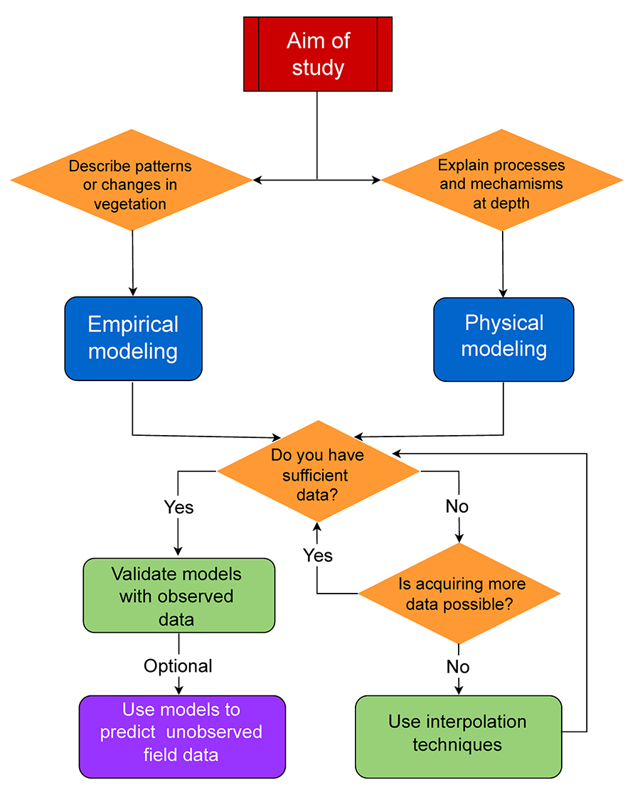
Figure 3. Flowchart for guiding the selection of the modeling approach in remote sensing-based vegetation studies. Two main approaches are distinguished: empirical modeling, aimed at describing patterns and changes in vegetation, and physical modeling, focused on explaining processes and mechanisms in depth. The choice depends mostly on the study goals, the availability of field data and the possibility of acquiring additional information. Interpolations techniques refer to the use of algorithms to estimate intermediate unobserved values between two observed values.

Figura 3. Diagrama de flujo para guiar la selección del enfoque de modelado en estudios de vegetación basados en teledetección. Se distinguen dos enfoques principales: modelado empírico, orientado a describir patrones y cambios en la vegetación, y modelado físico, enfocado en explicar procesos y mecanismos en profundidad. La elección depende fundamentalmente de los objeticos del estudio, la disponibilidad de datos de campo y la posibilidad de adquirir información adicional. Las técnicas de interpolación se refieren al uso de algoritmos para estimar valores intermedios no observados entre dos valores observados.

Table 1. Comparison of the characteristics, aims, strengths and weaknesses of the empirical and physical modeling approaches in remote sensing-based ecosystem studies.

Tabla 1. Comparación de las características, objetivos, fortalezas y debilidades de los enfoques empírico y físico de modelación en estudios de ecosistemas basados en la teledetección.

Characteristics	Empirical modeling	Physical modeling
Details needed	General studies: no detailed information from the study site is required	Detailed knowledge about the physical properties of the materials and their interactions with radiation is required
Complexity of implementation	Relatively easy to implement; standard computing requirements	Higher level of complexity and high computational requirements are needed to achieve precise results
Sensitivity to acquisition conditions	High temporal dependency on instantaneous conditions at the moment of image acquisition	Independence from instantaneous conditions at the moment of image acquisition
Generalization capacity	Limited generalization; mostly valid for the same or a similar study system	High generalization; may be applied to different conditions thus facilitating extrapolation to different environments
Data acquisition effort	Rapid acquisition of useful data for different objectives (generally mapping, assessment, and monitoring)	Acquisition of the necessary information to build the models is time consuming and cumbersome
Mechanistic understanding	The underlying mechanism of the model is unknown or unimportant	Understanding the underlying mechanism of the model is key
Dependency on training data	Highly dependent on training data; insufficient data cause reduced model performance	Lower dependency; these models can be calibrated with observed data, a process that is not comparable with training
Model adaptability	High adaptability; empirical models can be used in different sites and conditions with greater confidence	Limited adaptability; model parameters require adjustments to use it in different sites and conditions
Current level of use	Widely used in remote sensing-based vegetation studies	Still infrequently used in remote sensing-based vegetation studies
Scalability	High scalability; empirical models can be used across scales without strong restrictions.	Low scalability; physical models can only by used under the same conditions in which they were constructed.

Recognition of the limitations of empirical modeling led to the development of an alternative modeling approach known as physical modeling, which involves the construction of theoretical models based on the physical attributes of ecosystem features (Table 1). These theoretical models aim to understand as deeply as possible the nature of sources of radiation and their interaction with the environment (Sinclair et al., 1973; Myneni, 1991; Jacquemoud et al., 2000; Jiao et al., 2024). For this reason, the construction of physical models requires large amounts of specific data on variables that allow relating the physical characteristics of the system to its electromagnetic signals (Allen et al., 1969). Ultimately, the purpose of physical modeling is to produce detailed and specific knowledge of the modeled variables, as well as to establish causal relationships that explain the variation of ecosystem processes with the highest possible accuracy (Abdoun & El-Sekelly, 2017). In the case of plant communities, studies based on physical modeling consider multiple characteristics such as the spatial distribution of plants, their reflectance, illumination conditions, transmittance, absorption, and scattering of photons or electromagnetic waves, internal leaf tissue structure, the nature and concentration of pigments, chloroplast density, biochemical composition, and water content, among many others (Sinclair et al., 1973; Hosgood et al., 1994; Feldman, 2024).

Despite their importance for analyzing ecosystem processes, the development of physical models has not been limited to the study of plant communities but is also applied in other fields of knowledge, for example geology, civil engineering, and mining (Abdoun & El-Sekelly, 2017). All these types of studies explore elementary (static) processes on the surface to fully understand their characteristics and interactions, as well as to develop strategies for better understanding the observed phenomena. While these two goals may be achieved based on the same physical principles, it must be noted that modeling the surface for material identification is not comparable to modeling an ecological process (Kennedy et al., 2020). The latter involves highly dynamic relationships between variables that interact with each other, such as seasonality or humidity. These relationships increase the intrinsic complexity of the process and make it highly variable over short time intervals.

Notwithstanding their complexity, physical models offer attractive advantages over empirical models. For example, understanding the variation of the reflectance of a surface in relation to the terrain’s geometry can be done by simulating the interaction of light with the atmosphere and vegetation, a task that is accomplished by the DART (Discrete Anisotropic Radiative Transfer) model and the Bidirectional Reflectance Distribution Function (BRDF) (Gerard & North, 1997; Gastellu-Etchegorry et al., 2004). A further major advantage of physical modeling is its spatio-temporal independence; in this regard, a well-developed, highly complex physical model has the potential to build regional models applicable under different circumstances. Of course, integrating all the knowledge thus acquired involves a high degree of complexity (Prakash et al., 2017). Furthermore, having a large amount of detailed information does not guarantee success in modeling a process. Overall, physical modeling increases precision and the ability to describe a phenomenon in detail but requires specific resources (materials and instruments) to study the modeled variables more deeply. Additionally, the possibility of fully comprehending the interactions among model variables requires solid theoretical knowledge. For these reasons, the choice of the most useful approach to study ecosystem processes depends on the level of detail and scales involved (Woodcock & Strahler, 1987).

The comparison of the advantages and shortcomings of the two modeling approaches reviewed here explains why determining which is the best route for studying ecosystem processes is not straightforward. In fact, to consider the use of one or the other, it is necessary to have basic information about the system, its components, and its possible responses. Despite its limitations, empirical modeling has a proven ability to address problems that arise in parallel to the study of ecosystems. Furthermore, empirical models tackle the problem from a more practical perspective, focusing on modeling vegetation and its attributes without the necessity to understand the underlying mechanisms. By contrast, physical modeling aims for a more precise understanding of each variable considered, and, by doing so, it sheds light on the mechanisms involved in the terrain-image interactions by studying specific variables. Nevertheless, this is a time-consuming process, which represents a disadvantage in view of the accelerated deterioration of ecosystems and their processes, which requires immediate attention.

It has been suggested that physical modeling could eventually replace empirical modeling (e.g., Abdoun & El-Sekelly, 2017), but this claim may be unfounded as it overlooks important considerations related to the study of ecosystems. Although the examination of the main characteristics that distinguish the empirical and physical modeling approaches suggests that they are mutually exclusive, that is, that researchers should opt for one or the other in their studies, we envision a high potential for their combined use in remote sensing-based vegetation studies. On the one hand, both approaches can be conceived as complementary, since empirical modeling can contribute with case studies and identify research gaps, while physical modeling can provide the physical basis to understand the differences detected in these cases and facilitate a unifying comprehension. On the other hand, the combined application of the two modeling approaches can increase the precision of the predictions of vegetation attributes, which appears to be particularly effective in regions fraught with data scarcity (Zhou et al., 2023; Kumar et al., 2024; Liu et al., 2025). The integration of the two approaches has given rise to the emergence of a novel approach known as hybrid modeling (Schweidtmann et al., 2024).

Hybrid modeling takes advantage of the characteristics defining each approach synthesized in Table 1 and increases the explanatory capacity of the models through training processes, when using, for example, Machine Learning, while minimizing the limitations of each model taken individually (Zhou et al., 2023; Jiao et al., 2024). For example, the increased modeling precision associated to the physical approach may be offset by its high computational requirements and higher costs (Liu et al., 2025). In turn, empirical models are admittedly less precise, but they offer a much higher generalization potential in addition to their higher accessibility to many users due to its simplicity. In constructing physical models, the calculation of some parameters can be mathematically very complex, and in these cases, they may be replaced by coefficients obtained through empirical modeling. Likewise, empirical models could be used to fit the residuals of the physical models, which could result in physically sound models, but having higher predictive capacity and generalization potential than each of these models separately. However, the benefits from using a hybrid approach must not be overstated, as its inadequate use, for example, when the physical modeling component is not based on a sound knowledge of the physical nature of the studied elements, may result in reduced explanatory potential and modeling precision (Schweidtmann et al., 2024).

Conclusions

Several decades have elapsed since the introduction of remote sensing in ecosystem studies; however, innovations are still arising, offering new ways to understand the natural world and its processes. The two main approaches for modeling ecological attributes and processes through remote sensing (namely, empirical and physical modeling) contrasted in the last section of this review have different aims and neither one is superior nor more useful than the other. As is the case when selecting a given image spatial or spectral resolution, choosing a certain modeling approach for a remote sensing study always involves a trade-off between data precision and the efficiency in the use of resources, including time and data processing capabilities. Undoubtedly, studies focused on monitoring the spatial distribution of vegetation attributes and their changes over time, mostly conducted with an empirical approach, are invaluable from a practical perspective. On the contrary, physical modeling is rather geared toward gaining a deeper understanding of the relationship between surface properties, illumination characteristics, and remote-sensed variables. More importantly, however, it is increasingly evident that these approaches are not mutually exclusive, as it combined use (represented by the emergent hybrid modeling approach) makes the most of each of them while overcoming some of their drawbacks, all of which results in much more precise and efficient modeling. By viewing the two approaches as complementary research tools, we may be better able to address pressing needs in ecosystem monitoring. Of course, the future development of hybrid modeling faces important challenges, and future research avenues should focus on issues such as the feasibility of scaling hybrid models, or their transferability across ecosystems.

Authors’ contributions

Daniel Chávez: Conceptualization, investigation, writing-first draft, writing-review and editing. Jonatan V. Solórzano: Investigation, writing-review and editing. Jorge A. Meave: Conceptualization, investigation, writing-review and editing.

Data and code availability

This paper does not use original datasets.

Financing, required permits, potential conflicts of interest and acknowledgments

This study was funded by SECIHTI, the Mexican Ministry of Science, Humanities, Technology and Innovation (formely CONACyT, The National Council of Science and Technology of Mexico). This paper constitutes a partial fulfillment of the Programa de Doctorado del Posgrado en Ciencias Biológicas, Universidad Nacional Autónoma de México. D.C. received a doctoral scholarship from CONACyT.

The authors do not have any financial or personal conflict of interest to declare related to the information and presentation of this paper.

We are grateful to Abril Chávez and Marco A. Romero-Romero for figure preparation.

References

Abdoun, T., & El-Sekelly, W. (2017). Recent advances in physical modeling and remote sensing of civil infrastructure systems. Innovative Infrastructure Solutions, 2, 44. https://doi.org/10.1007/s41062-017-0078-3

Adam, E., Mutanga, O., & Rugege, D. (2009). Multispectral and hyperspectral remote sensing for identification and mapping of wetland vegetation: A review. Wetlands Ecology and Management, 18, 281–296. https://doi.org/10.1007/s11273-009-9169-z

Adjovu, G. E., Stephen, H., James, D., & Ahmad, S. (2023). Overview of the application of remote sensing in effective monitoring of water quality parameters. Remote Sensing, 15(7), 1938. https://doi.org/10.3390/rs15071938

Ahmad, A., Gilani, H., & Ahmad, S. R. (2021). Forest aboveground biomass estimation and mapping through high-resolution optical satellite imagery: A literature review. Forests, 12(7), 914. https://doi.org/10.3390/f12070914

Allen, W. A., Gausman, H. W., Richardson, A. J., & Thomas, J. R. (1969). Interaction of isotropic light with a compact plant leaf. Journal of the Optical Society of America, 39, 1376–1379. https://doi.org/10.1364/JOSA.59.001376

Alvarez-Vanhard, E., Corpetti, T., & Houet, T. (2021). UAV & satellite synergies for optical remote sensing applications: A literature review. Science of Remote Sensing, 3, 100019. https://doi.org/10.1016/j.srs.2021.100019

Anderson, K., & Gaston, K. J. (2013). Lightweight unmanned aerial vehicles will revolutionize spatial ecology. Frontiers in Ecology and the Environment, 11(3), 138–146. https://doi.org/10.1890/120150

Anyomi, K. A., Neary, B., Chen, J., & Mayor, S. J. (2022). A critical review of successional dynamics in boreal forest of North America. Environmental Reviews, 30(4), 563–594. https://doi.org/10.1139/er-2021-0106

Aplin, P. (2004). Remote sensing: Land cover. Progress in Physical Geography, 28, 283–293. https://doi.org/10.1191/0309133304pp413pr

Aquino, C., Mitchard, E. T. A., McNicol, I. M., Carstairs, H., Burt, A., Vilca, B. L. P., … Disney, M. (2025). Detecting selective logging in tropical forests with optical satellite data: An experiment in Peru shows texture at 3 m gives the best results. Remote Sensing in Ecology and Conservation, 11, 100–118. https://doi.org/10.1002/rse2.414

Aschbacher, J., Ofren, R., Delsol, J. P., Suselo, T. B., Vibulsresth, S., & Charrupat, T. (1995). An integrated comparative approach to mangrove vegetation mapping using advanced remote sensing and GIS technologies: Preliminary results. Hydrobiologia, 295, 285–294. https://doi.org/10.1007/BF00029135

Asner, G. P., & Heidebrecht, K. B. (2002). Spectral of vegetation, soil and dry carbon cover in arid regions: Comparing multispectral and hyperspectral observations. International Journal of Remote Sensing, 23, 3939–3958. https://doi.org/10.1080/01431160110115960

Asner, G. P., Scurlock, J. M. O., & Hicke, J. A. (2003). Global synthesis of leaf area index observations: Implications for ecological and remote sensing studies. Global Ecology and Biogeography, 12(3), 191–205. https://doi.org/10.1046/j.1466-822X.2003.00026.x

Atkinson, P., & Aplin, P. (2004). Spatial variation in land cover and choice of spatial resolution for remote sensing. International Journal of Remote Sensing, 25, 3687–3702. https://doi.org/10.1080/01431160310001654383

Barbier, N., Couteron, P., Gastellu-Etchegorry, J. P., & Proisy, C. (2012). Linking canopy images to forest structural parameters: Potential of a modeling framework. Annals of Forest Science, 69, 305–311. https://doi.org/10.1007/s13595-011-0116-9

Barbier, N., & Couteron, P. (2015). Attenuating the bidirectional texture variation of satellite images of tropical forest canopies. Remote Sensing of Environment, 171, 245–260. https://doi.org/10.1016/j.rse.2015.10.007

Barbosa, J. M., Broadbent, E. N., & Bitencourt, M. D. (2014). Remote sensing of aboveground biomass in tropical secondary forests: A review. International Journal of Forestry Research, 2014, 715796. https://doi.org/10.1155/2014/715796

Bastin, J.-F. F., Barbier, N., Couteron, P., Adams, B., Shapiro, A., Bogaert, J., & de Cannière, C. (2014). Aboveground biomass mapping of African forest mosaics using canopy texture analysis: Towards a regional approach. Ecological Applications, 24(8), 1984–2001. https://doi.org/10.1890/13-1574.1

Bennett, A. F., Haslem, A., Cheal, D. C., Clarke, M. F., Jones, R. N., Koehn, J. D., … Yen, A. L. (2009). Ecological processes: A key element in strategies for nature conservation. Ecological Management & Restoration, 10, 192–199. https://doi.org/10.1111/j.1442-8903.2009.00489.x

Blasco, F., Gauquelin, T., Rasolofoharinoro, M., Denis, J., Aizpuru, M., & Caldairou, V. (1998). Recent advances in mangrove studies using remote sensing data. Marine and Freshwater Research, 49, 287–296. https://doi.org/10.1071/MF97153

Block, S., González, E. J., Gallardo-Cruz, J. A., Fernández, A., Solórzano, J. V., & Meave, J. A. (2016). Using Google Earth surface metrics to predict plant species richness in a complex landscape. Remote Sensing, 8, 865. https://doi.org/10.3390/rs8100865

Bongers, F. (2001). Methods to assess tropical rain forest canopy structure: An overview. Plant Ecology, 153, 263–277. https://doi.org/10.1023/A:1017555605618

Borgonovo, E., Tarantola, S., Plischke, E., & Morris, M. D. (2014). Transformations and invariance in the sensitivity analysis of computer experiments. Journal of the Royal Statistical Society Series B: Statistical Methodology, 76, 925–947. https://doi.org/10.1111/rssb.12052

Bramich, J., Bolch, C. J. S., & Fischer, A. (2021). Improved red-edge chlorophyll-a detection for Sentinel 2. Ecological Indicators, 120, 106876. https://doi.org/10.1016/j.ecolind.2020.106876

Bruniquel-Pinel, V., & Gastellu-Etchegorry, J. P. (1998). Sensitivity of texture of high resolution images of forest to biophysical and acquisition parameters. Remote Sensing of Environment, 65(1), 61–85. https://doi.org/10.1016/S0034-4257(98)00009-1

Bürkner, P.-C., Gabry, J., & Vehtari, A. (2020). Approximate leave-future out cross-validation for Bayesian time series models. Journal of Statistical Computation and Simulation, 90(14), 2499–2523. https://doi.org/10.1080/00949655.2020.1783262

Butler, S., & O'Dwyer, J. P. (2020). Cooperation and stability for complex systems in resource-limited environments. Theoretical Ecology, 13, 239–250. https://doi.org/10.1007/s12080-019-00447-5

Cadenasso, M. L., Pickett, S. T. A., Weathers, K. C., & Jones, C. G. (2003). A framework for a theory of ecological boundaries. BioScience, 53, 750–758. https://doi.org/10.1641/0006-3568(2003)053[0750:AFFATO]2.0.CO;2

Campbell, G. S., & Norman, J. M. (1989). The description and measurement of plant canopy structure. In G. Russell, B. Marshall, & P. G. Jarvis (Eds.), Plant canopies: Their growth, form and function (pp. 1–20). Cambridge University Press. https://doi.org/10.1017/CBO9780511752308.002

Camps-Valls, G., Tuia, D., Gómez-Chova, L., Jiménez, S., & Malo, J. (2012). Remote sensing image processing. Morgan & Claypool Publishers. https://doi.org/10.1007/978-3-031-02247-0

Cavender-Bares, J., Schneider, F. D., Santos, M. J., Armstrong, A., Carnaval, A., Dahlin, K. M., … Wilson, A. M. (2022). Integrating remote sensing with ecology and evolution to advance biodiversity conservation. Nature Ecology & Evolution, 6, 506–519. https://doi.org/10.1038/s41559-022-01702-5

Chávez, D., López-Portillo, J., Gallardo-Cruz, J. A., & Meave, J. A. (2024). Approaches, potential, and challenges in the use of remote sensing to study mangrove and other tropical wetland forests. Botanical Sciences, 102(1), 1–25. https://doi.org/10.17129/botsci.3358

Chinea, J. D. (2002). Teledetección de bosques tropicales. In M. R. Guariguata & G. H. Kattan (Eds.), Ecología de bosques neotropicales. Libro Universitario Regional.

Chuvieco, E. (2016). Fundamentals of satellite remote sensing: An environmental approach (2nd ed.). CRC Press. https://doi.org/10.1201/b19478

Clausi, D. A., & Zhao, Y. (2002). Rapid extraction of image texture by co-occurrence using a hybrid data structure. Computers & Geosciences, 28(6), 763–774. https://doi.org/10.1016/S0098-3004(01)00108-X

Connell, J. H., & Slatyer, R. O. (1977). Mechanisms of succession in natural communities and their role in community stability and organization. The American Naturalist, 111, 1119–1144. https://doi.org/10.1086/283241

Couteron, P. (2002). Quantifying change in patterned semi-arid vegetation by Fourier analysis of digitized aerial photographs. International Journal of Remote Sensing, 17, 3407–3425. https://doi.org/10.1080/01431160110107699

Couteron, P., Pelissier, R., Nicolini, E. A., & Paget, D. (2005). Predicting tropical forest stand structure parameters from Fourier transform of very high-resolution remotely sensed canopy images. Journal of Applied Ecology, 42, 1121–1128. https://doi.org/10.1111/j.1365-2664.2005.01097.x

Crawley, M. J. (1997). Plant ecology (2nd ed.). Blackwell. https://doi.org/10.1002/9781444313642

Culbert, P. D., Pidgeon, A. M., St.-Louis, V., Bash, D., & Radeloff, V. C. (2009). The impact of phenological variation on texture measures of remotely sensed imagery. IEEE Journal of Selected Topics in Applied Earth Observations and Remote Sensing, 2(4), 299–309. https://doi.org/10.1109/JSTARS.2009.2021959

Daleo, P., Alberti, J., Chaneton, E. J., Iribarne, O., Tognetti, P. M., Bakker, J. D., … Hautier, Y. (2023). Environmental heterogeneity modulates the effect of plant diversity on the spatial variability of grassland biomass. Nature Communications, 14, 1809. https://doi.org/10.1038/s41467-023-37395-y

Dansereau, P. (1957). Biogeography: An ecological perspective. The Ronald Press.

Delegido, J., Verrelst, J., Alonso, L., & Moreno, J. (2011). Evaluation of Sentinel-2 red-edge bands for empirical estimation of green LAI and chlorophyll content. Sensors, 11(7), 7063–7081. https://doi.org/10.3390/s110707063

Dozier, J., Bair, E. H., Baskaran, L., Brodrick, P. G., Carmon, N., Kokaly, R. F., … Thompson, D. R. (2022). Error and uncertainty degrade topographic corrections of remotely sensed data. JGR Biogeosciences, 127(11), e2022JG007147. https://doi.org/10.1029/2022JG007147

Dronova, I., & Taddeo, S. (2022). Remote sensing of phenology: Towards the comprehensive indicators of plant community dynamics from species to regional scales. Journal of Ecology, 110(7), 1460–1484. https://doi.org/10.1111/1365-2745.13897

Du, R., Lu, J., Xiang, Y., Zhang, F., Chen, J., Tang, Z., Shi, H., Wang, X., & Li, W. (2024). Estimation of winter canola growth parameter from UAV multi-angular spectral-texture information using stacking-based ensemble learning model. Computers and Electronics in Agriculture, 222, 109074. https://doi.org/10.1016/j.compag.2024.109074

Dube, T., Onisimo, M., Cletah, S., Adelabu, S., & Tsitsi, B. (2016). Remote sensing of aboveground forest biomass: A review. Tropical Ecology, 57(2), 125–132.

Eckert, S. (2012). Improved forest biomass and carbon estimations using texture measures from WorldView-2 satellite data. Remote Sensing, 4, 810–829. https://doi.org/10.3390/rs4040810

Eide, A., Koparan, C., Zhang, Y., Ostlie, M., Howatt, K., & Sun, X. (2021). UAV-assisted thermal infrared and multispectral imaging of weed canopies for glyphosate resistance detection. Remote Sensing, 13, 4606. https://doi.org/10.3390/rs13224606

Einzmann, K., Atzberger, C., Pinnel, N., Glas, C., Böck, S., Seitz, R., & Immitzer, M. (2021). Early detection of spruce vitality loss with hyperspectral data: Results of an experimental study in Bavaria, Germany. Remote Sensing of Environment, 266, 112676. https://doi.org/10.1016/j.rse.2021.112676

Farwell, L. S., Gudex-Cross, D., Anise, I. E., Bosch, M. J., Olah, A. M., … Pidgeon, A. M. (2021). Satellite image texture captures vegetation heterogeneity and explains patterns of bird richness. Remote Sensing of Environment, 253, 112175. https://doi.org/10.1016/j.rse.2020.112175

Fassnacht, F. E., White, J. C., Wulder, M. A., & Næsset, E. (2024). Remote sensing in forestry: Current challenges, considerations and directions. Forestry: An International Journal of Forest Research, 97, 11–37. https://doi.org/10.1093/forestry/cpad024

Fatoyinbo, T. E., & Armstrong, A. H. (2010). Remote characterization of biomass measurements: Case study of mangrove forest. In M. Momba & F. Bux (Eds.), Biomass. Sciyo.

Fatoyinbo, T. E., Simard, M., Washington-Allen, R. A., & Shugart, H. H. (2008). Landscape-scale extent, height, biomass, and carbon estimation of Mozambique's mangrove forests with Landsat ETM+ and Shuttle. Journal of Geophysical Research, 113, G02S06. https://doi.org/10.1029/2007JG000551

Feldman, A. F. (2024). Emerging methods to validate remotely sensed vegetation. Geophysical Research Letters, 51(14), e2024GL110505. https://doi.org/10.1029/2024GL110505

Feng, Q., Liu, J., & Gong, J. (2015). UAV remote sensing for urban vegetation mapping using random forest and texture analysis. Remote Sensing, 7(1), 1074–1094. https://doi.org/10.3390/rs70101074

Fernández-Manso, A., Fernández-Manso, O., & Quintano, C. (2016). SENTINEL-2A red-edge spectral indices suitability for discriminating burn severity. International Journal of Applied Earth Observation and Geoinformation, 50, 170–175. https://doi.org/10.1016/j.jag.2016.03.005

Fernández-Pacheco, V. M., Amezqueta-García, A., & Álvarez-Álvarez, E. (2023). Análisis de la evolución del complejo dunar Salinas - El Espartal mediante el empleo de ortofotografía, DSAS y lidar (1957–2021). Ingeniería del Agua, 27, 223–235. https://doi.org/10.4995/ia.2023.20021

Fichot, C. G., Tzortziou, M., & Mannino, A. (2023). Remote sensing of dissolved organic carbon (DOC) stocks, fluxes and transformations along the land-ocean aquatic continuum: Advances, challenges, and opportunities. Earth-Science Reviews, 242, 104446. https://doi.org/10.1016/j.earscirev.2023.104446

Fleming, A., Conway, T. M., Sleightholm, P., & McKay, J. (2025). Aerial imagery as a tool for monitoring urban tree retention: Applications, strengths and challenges for backyard tree planting programs. Arboriculture & Urban Forestry, 51, 022. https://doi.org/10.48044/jauf.2025.022

Foody, G. M. (2003). Remote sensing of tropical forest environments: Towards the monitoring of environmental resources for sustainable development. International Journal of Remote Sensing, 24, 4035–4046. https://doi.org/10.1080/0143116031000103853

Foody, G. M., & Cutler, M. (2001). Mapping the biomass of Bornean tropical rain forest from remotely sensed data. Global Ecology and Biogeography, 10, 379–387. https://doi.org/10.1046/j.1466-822X.2001.00248.x

Gallardo-Cruz, J. A., Meave, J. A., González, E. J., Lebrija-Trejos, E., Romero-Romero, M. A., Pérez-García, E. A., … Martorell, C. (2012). Predicting tropical dry forest successional attributes from space: Is the key hidden in image texture? PLOS ONE, 7, e30506. https://doi.org/10.1371/journal.pone.0030506

Gallardo-Cruz, J. A., Solórzano, J. V., González, E. J., & Meave, J. A. (2024). The effect of spatial scale on the prediction of tropical forest attributes from image texture. International Journal of Forestry Research, 2024, 7178211. https://doi.org/10.1155/2024/7178211

Gamon, J. A., Peñuelas, J., & Field, C. B. (1992). A narrow-waveband spectral index that tracks diurnal changes in photosynthetic efficiency. Remote Sensing of Environment, 41(1), 35–44. https://doi.org/10.1016/0034-4257(92)90059-S

Gamon, J. A., Huemmrich, K. F., Wong, C. Y. S., Ensminger, I., Garrity, S., Hollinger, D. Y., … Peñuelas, J. (2016). A remotely sensed pigment index reveals photosynthetic phenology in evergreen conifers. Proceedings of the National Academy of Sciences of the United States of America, 113(46), 13087–13092. https://doi.org/10.1073/pnas.1606162113

García, M., Saatchi, S., Ustin, S., & Balzter, H. (2018). Modelling forest canopy height by integrating airborne LiDAR samples with satellite radar and multispectral imagery. International Journal of Applied Earth Observation and Geoinformation, 66, 159–173. https://doi.org/10.1016/j.jag.2017.11.017

Gao, B. (1996). NDWI: A normalized difference water index for remote sensing of vegetation liquid water from space. Remote Sensing of Environment, 58, 257–266. https://doi.org/10.1016/S0034-4257(96)00067-3

Gastellu-Etchegorry, J. P., Martin, E., & Gascon, F. (2004). DART: A 3D model for simulating satellite images and studying surface radiation budget. International Journal of Remote Sensing, 25(1), 73–96. https://doi.org/10.1080/0143116031000115166

Gerard, F. F., & North, P. R. J. (1997). Analyzing the effect of structural variability and canopy gaps on forest BRDF using a geometric-optical model. Remote Sensing of Environment, 62(1), 46–62. https://doi.org/10.1016/S0034-4257(97)00070-9

Gitelson, A. A., & Merzlyak, M. (1994). Spectral reflectance changes associated with autumn senescence of Aesculus hippocastanum L. and Acer platanoides L. leaves: Spectral features and relation to chlorophyll estimation. Journal of Plant Physiology, 143, 286–292. https://doi.org/10.1016/S0176-1617(11)81633-0

Gitelson, A. A., Gritz, Y., & Merzlyak, M. (2003). Relationships between leaf chlorophyll content and spectral reflectance and algorithms for non-destructive chlorophyll assessment in higher plant leaves. Journal of Plant Physiology, 160, 271–282. https://doi.org/10.1078/0176-1617-00887

Guan, K., Wood, E. F., & Caylor, K. K. (2012). Multi-sensor derivation of regional vegetation fractional cover in Africa. Remote Sensing of Environment, 124, 653–665. https://doi.org/10.1016/j.rse.2012.06.005

Haralick, R. M. (1979). Statistical and structural approaches to texture. Proceedings of the Institute of Electrical and Electronics Engineers, 67, 786–804. https://doi.org/10.1109/PROC.1979.11328

Haralick, R. M., Shanmugam, K., & Dinstein, I. (1973). Textural features for image classification. IEEE Transactions on Systems, Man, and Cybernetics, 3, 610–621. https://doi.org/10.1109/TSMC.1973.4309314

Harrison, P. A., Berry, P. M., Simpson, G., Haslett, J. R., Blicharska, M., Bucur, M., … Turkelboom, F. (2014). Linkages between biodiversity attributes and ecosystem services: A systematic review. Ecosystem Services, 9, 191–203. https://doi.org/10.1016/j.ecoser.2014.05.006

Hillier, F. S., & Lieberman, G. (1990). Introduction to operations research (5th ed.). McGraw-Hill.

Horler, D. N. H., Dockray, M., & Barber, J. (1983). The red edge of plant leaf reflectance. International Journal of Remote Sensing, 4, 273–288. https://doi.org/10.1080/01431168308948546

Hossain, M. S., & Lin, K. (2003). Remote sensing and GIS applications for suitable mangrove afforestation area selection in the coastal zone of Bangladesh. Geocarto International, 18, 61–65. https://doi.org/10.1080/10106040308542264

Hosgood, B., Jacquemoud, S., Andreoli, G., Verdebout, J., Pedrini, G., & Schmuck, G. (1994). Leaf optical properties experiment 93 (LO-PEX93). European Commission, Joint Research Centre, Institute for Remote Sensing Applications. Report EUR 16095.

Huete, A. R. (1988). A soil-adjusted vegetation index (SAVI). Remote Sensing of Environment, 23, 295–309. https://doi.org/10.1016/0034-4257(88)90106-X

Huete, A. R., Liu, H. Q., Batchily, K., & van Leeuwen, W. (1997). A comparison of vegetation indices over a global set of TM images for EOS-MODIS. Remote Sensing of Environment, 59(3), 440–451. https://doi.org/10.1016/S0034-4257(96)00112-5

Huston, M. A. (1994). Biological diversity: The coexistence of species on changing landscapes. Cambridge University Press.

Ibarra-Manríquez, G., González-Espinosa, M., Martínez-Ramos, M., & Meave, J. A. (2022). From vegetation ecology to vegetation science: Current trends and perspectives. Botanical Sciences, 100(Special Issue), S137–S174. https://doi.org/10.17129/botsci.3171

Iqbal, I. M., Balzter, H., Bareen, F., & Shabbir, A. (2021). Identifying the spectral signatures of invasive and native plant species in two protected areas of Pakistan through field spectroscopy. Remote Sensing, 13(19), 4009. https://doi.org/10.3390/rs13194009

Islam, K. I., Elias, E., Carroll, K. C., & Brown, C. (2023). Exploring random forest machine learning and remote sensing data for streamflow prediction: An alternative approach to a process-based hydrologic modeling in a snowmelt-driven watershed. Remote Sensing, 15(16), 3999. https://doi.org/10.3390/rs15163999

Jacquemoud, S., Bacour, C., Poilvé, H., & Frangi, J. P. (2000). Comparison of four radiative transfer models to simulate plant canopies reflectance: Direct and inverse mode. Remote Sensing of Environment, 74, 471–481. https://doi.org/10.1016/S0034-4257(00)00139-5

Jensen, J. R. (1983). Urban/suburban land use analysis. In R. N. Colwell (Ed.), Manual of remote sensing (2nd ed.). American Society of Photogrammetry.

Jensen, J. R. (2007). Remote sensing of the environment: An earth resource perspective (2nd ed.). Pearson Prentice Hall.

Jiao, S., Li, Z., Gai, J., Zou, L., & Su, Y. (2024). Hybrid physics-machine learning models for predicting rate of penetration in the Halahatang oil field, Tarim Basin. Scientific Reports, 14, 5957. https://doi.org/10.1038/s41598-024-56640-y

Jones, H. G., & Vauhgan, R. A. (2010). Remote sensing of vegetation: Principles, techniques, and applications. Oxford University Press.

Kayitakire, F., Hamel, C., & Defourny, P. (2006). Retrieving forest structure variables based on image texture analysis and IKONOS-2 imagery. Remote Sensing of Environment, 102, 390–401. https://doi.org/10.1016/j.rse.2006.02.022

Kennedy, B. E., King, D. J., & Duffe, J. (2020). Comparison of empirical and physical modelling for estimation of biochemical and biophysical vegetation properties: Field scale analysis across an arctic bioclimatic gradient. Remote Sensing, 12(18), 3073. https://doi.org/10.3390/rs12183073

Kershaw, K. A., & Looney, J. H. H. (1985). Quantitative and dynamic plant ecology (3rd ed.). Edward Arnold.

Kenneth-Shultis, J., & Myneni, R. B. (1988). Radiative transfer in vegetation canopies with anisotropic scattering. Journal of Quantitative Spectroscopy & Radiative Transfer, 39, 115–129. https://doi.org/10.1016/0022-4073(88)90079-9

Kent, M. (2012). Vegetation description and analysis: A practical approach (2nd ed.). Wiley-Blackwell.

Kiltie, R. A., Fan, J., & Laine, A. F. (1995). A wavelet-based metric for visual texture discrimination with applications in evolutionary ecology. Mathematical Biosciences, 126(1), 21–39. https://doi.org/10.1016/0025-5564(94)00034-W

Kirk, J. T. O. (1984). Dependence of relationship between inherent and apparent optical properties of water on solar altitude. Limnology and Oceanography, 29, 350–356. https://doi.org/10.4319/lo.1984.29.2.0350

Knudby, A. (2021). Remote sensing. Creative Commons.

Kothari, S., & Schweiger, A. K. (2022). Plant spectra as integrative measures of plant phenotypes. Journal of Ecology, 110(11), 2536–2554. https://doi.org/10.1111/1365-2745.13972

Kötz, B., Schaepman, M., Morsdorf, F., Bowyer, P., Itten, K., & Allgöwer, B. (2024). Radiative transfer modeling within a heterogeneous canopy for estimation of forest fire fuel properties. Remote Sensing of Environment, 92(3), 332–344. https://doi.org/10.1016/j.rse.2004.05.015

Kuenzer, C., Bluemel, A., Gebhardt, S., Quoc, T. V., & Dech, S. (2011). Remote sensing of mangrove ecosystems: A review. Remote Sensing, 3(5), 878–928. https://doi.org/10.3390/rs3050878

Kumar, S., Choudhary, M. K., & Thomas, T. (2024). A hybrid technique to enhance the rainfall-runoff prediction of physical and data-driven model: A case study of Upper Narmanda River Sub-basin, India. Scientific Reports, 14, 26263. https://doi.org/10.1038/s41598-024-77655-5

Lalechère, E., Monnet, J.-M., Breen, J., & Fuhr, M. (2024). Assessing the potential of remote sensing-based models to predict old-growth forests on large spatiotemporal scales. Journal of Environmental Management, 351, 119865. https://doi.org/10.1016/j.jenvman.2023.119865

LaRue, E. A., Hardiman, B. S., Elliott, J. M., & Fei, S. (2019). Structural diversity as a predictor of ecosystem function. Environmental Research Letters, 14, 114011. https://doi.org/10.1088/1748-9326/ab49bb

Lausch, A., Bastian, O., Klotz, S., Leitão, P. J., Jung, A., Rocchini, D., … Knapp, S. (2018). Understanding and assessing vegetation health by in situ species and remote-sensing approaches. Methods in Ecology and Evolution, 9(8), 1799–1809. https://doi.org/10.1111/2041-210X.13025

Lebrija-Trejos, E., Pérez-García, E. A., Meave, J. A., Poorter, L., & Bongers, F. (2011). Environmental changes during secondary succession in a tropical dry forest in Mexico. Journal of Tropical Ecology, 27, 477–489. https://doi.org/10.1017/S0266467411000253

Leduc, M.-B., & Knudby, J. A. (2018). Mapping wild leek through the forest canopy using UAV. Remote Sensing, 10, 70. https://doi.org/10.20381/ruor-23313

Lee, D. K. (2020). Data transformation: A focus on the interpretation. Korean Journal of Anesthesiology, 73(6), 503–508. https://doi.org/10.4097/kja.20137

Legendre, P. (1993). Spatial autocorrelation: Trouble or new paradigm? Ecology, 74(6), 1659–1673. https://doi.org/10.2307/1939924

Li, C., Czyż, E. A., Halitschke, R., Baldwin, I. T., Schaepman, M. E., & Schuman, M. C. (2023). Evaluating potential of leaf reflectance spectra to monitor plant genetic variation. Plant Methods, 19, 108. https://doi.org/10.1186/s13007-023-01089-9

Li, J., Liao, C., Zhang, W., Fu, H., & Fu, S. (2022). UAV path planning model based on R5DOS model improved A-star algorithm. Applied Sciences, 12(22), 11338. https://doi.org/10.3390/app122211338

Lian, Z., Wang, J., Fan, C., & van Gadow, K. (2022). Structure complexity is the primary driver of functional diversity in the temperate forests of northeastern China. Forest Ecosystems, 9, 100048. https://doi.org/10.1016/j.fecs.2022.100048

Lillesand, T. M., Kiefer, R. W., & Chipman, J. W. (2015). Remote sensing and image interpretation. John Wiley & Sons.

Lin, N., Zhang, D., Feng, S., Ding, K., Tan, L., Wang, B., … Tang, F. (2023). Rapid landslide extraction from high-resolution remote sensing images using SHAP-OPT-XGBoost. Remote Sensing, 15(8), 2107. https://doi.org/10.3390/rs15082107

Liu, Y., Fan, Y., Feng, H., Chen, R., Bian, M., Ma, Y., … Yang, G. (2024). Estimating potato above-ground biomass based on vegetation indices and texture features constructed from sensitive bands of UAV hyperspectral imagery. Computers and Electronics in Agriculture, 220, 108918. https://doi.org/10.1016/j.compag.2024.108918

Liu, W., Mo, L., Li, X., Xiao, W., Huang, H., & Zhang, Y. (2025). A hybrid deep learning rainfall-runoff forecasting model incorporating spatiotemporal information from multi-source data. Expert Systems with Applications, 298, 129974. https://doi.org/10.1016/j.eswa.2025.129974

Lu, D., & Batistella, M. (2005). Exploring TM image texture and its relationships with biomass estimation in Rondônia, Brazilian Amazon. Acta Amazonica, 35(2), 249–257. https://doi.org/10.1590/S0044-59672005000200015

Lyu, X., Li, X., Dang, D., Dou, H., Wang, K., & Lou, A. (2022). Unmanned aerial vehicle (UAV) remote sensing in grassland ecosystem monitoring: A systematic review. Remote Sensing, 14(5), 1096. https://doi.org/10.3390/rs14051096

Ma, L., Liu, Y., Zhang, X., Ye, Y., Yin, G., & Johnson, B. A. (2019). Deep learning in remote sensing applications: A meta-analysis and review. ISPRS Journal of Photogrammetry and Remote Sensing, 152, 166–177. https://doi.org/10.1016/j.isprsjprs.2019.04.015

Magurran, A. E. (2004). Measuring biological diversity. Blackwell Science.

Manzo-Delgado, L., & Meave, J. A. (2003). La vegetación vista desde el espacio: La fenología foliar a través de la percepción remota. Ciencia, 54, 18–28.

Margules, C., & Sarkar, S. (2009). Planeación sistemática de la conservación. Universidad Nacional Autónoma de México.

McCoy, E. D., & Bell, S. S. (1991). Habitat structure: The evolution and diversification of a complex topic. In S. S. Bell, E. D. McCoy, & H. R. Mushinsky (Eds.), Habitat structure: The physical arrangement of objects in space (pp. 3–27). Springer. https://doi.org/10.1007/978-94-011-3076-9_1

Meave, J. A., & Pérez-García, E. A. (2013). Vegetación: Caracterización y factores que determinan su distribución. In: J. Márquez-Guzmán, M. Collazo-Ortega, M. Martínez-Gordillo, A. Orozco-Segovia, & S. Vázquez-Santana (Eds.), Biología de angiospermas.

Mejía-Domínguez, N. R., Meave, J. A., Díaz-Ávalos, C., & González, E. J. (2011). Individual canopy-tree species effects on their immediate understory microsite and sapling community dynamics. Biotropica, 43(5), 572–581. https://doi.org/10.1111/j.1744-7429.2010.00739.x

Merzlyak, J. R., Gitelson, A. A., Chivkunova, O. B., & Rakitin, V. Y. (1999). Non-destructive optical detection of pigment changes during leaf senescence and fruit ripening. Physiologia Plantarum, 106, 135–141. https://doi.org/10.1034/j.1399-3054.1999.106119.x

Mezaal, M. R., Pradhan, B., Shafri, H. Z. M., & Yusoff, Z. M. (2017). Automatic landslide detection using Dempster-Shafer theory from LiDAR-derived data and orthophotos. Geomatics, Natural Hazards and Risk, 8, 1935–1954. https://doi.org/10.1080/19475705.2017.1401013

Morgan, J., Gergel, S. E., & Coops, N. C. (2010). Aerial photography: A rapidly evolving tool for ecological management. BioScience, 60(1), 47–59. https://doi.org/10.1525/bio.2010.60.1.9

Morin, P. J. (1999). Community ecology. Wiley-Blackwell.

Morin, D., Planells, M., Guyon, D., Villard, L., Mermoz, S., Bouvet, A., … Dedieu, G. (2019). Estimation and mapping of forest structure parameters from open access satellite images: Development of a generic method with a study case on coniferous plantation. Remote Sensing, 11(11), 1275. https://doi.org/10.3390/rs11111275

Mueller-Dombois, D., & Ellenberg, H. (1974). Aims and methods of vegetation ecology. Wiley & Sons.

Myint, S. W., Gober, P., Brazel, A., Grossman-Clarke, S., & Weng, Q. (2011). Per-pixel vs. object-based classification of urban land cover extraction using high spatial resolution imagery. Remote Sensing of Environment, 115, 1145–1161. https://doi.org/10.1016/j.rse.2010.12.017

Myneni, R. B. (1991). Modeling radiative transfer and photosynthesis in three-dimensional vegetation canopies. Agricultural and Forest Meteorology, 55, 323–344. https://doi.org/10.1016/0168-1923(91)90069-3

Myneni, R., Maggion, S., Iaquinta, J., Privette, J. L., Gobron, N., Pinty, B., … Williams, D. L. (1995). Optical remote sensing of vegetation: Modeling, caveats, and algorithms. Remote Sensing of Environment, 51, 169–188. https://doi.org/10.1016/0034-4257(94)00073-V

Nagendra, H., & Rocchini, D. (2008). High resolution satellite imagery for tropical biodiversity studies: The devil is in the detail. Biodiversity and Conservation, 17, 3431–3442. https://doi.org/10.1007/s10531-008-9479-0

Navulur, K. (2007). Multispectral image analysis using the object-oriented paradigm. CRC Press. https://doi.org/10.1201/9781420043075

Norman, J. M., & Campbell, G. S. (1989). Canopy structure. In R. W. Pearcy, J. R. Ehleringer, H. A. Mooney, & P. W. Rundel (Eds.), Plant physiological ecology (pp. xx–xx). Springer. https://doi.org/10.1007/978-94-009-2221-1_14

Obata, K., Miura, T., & Yoshioka, H. (2012). Analysis of the scaling effects in the area-averaged fraction of vegetation cover retrieved using an NDVI-isoline-based linear mixture model. Remote Sensing, 4(7), 2156–2180. https://doi.org/10.3390/rs4072156

Ohmann, J. L., & Gregory, M. J. (2002). Predictive mapping of forest composition and structure with direct gradient analysis and nearest-neighbor imputation in coastal Oregon, U.S.A. Canadian Journal of Forest Research, 32, 725–741. https://doi.org/10.1139/x02-011

Ozdemir, I., & Karnieli, A. (2011). Predicting forest structural parameters using the image texture derived from WorldView-2 multispectral imagery in a dryland forest, Israel. International Journal of Applied Earth Observation and Geoinformation, 13, 701–710. https://doi.org/10.1016/j.jag.2011.05.006

Parker, G. G., Fitzjarrald, D. R., & Sampaio, I. C. G. (2019). Consequences of environmental heterogeneity for the photosynthetic light environment of a tropical forest. Agricultural and Forest Meteorology, 278, 107661. https://doi.org/10.1016/j.agrformet.2019.107661

Peña, L., Rentería, V., Velásquez, C., Ojeda, M. L., & Barrera, E. (2019). Absorbancia y reflectancia de hojas de Ficus contaminadas con nanopartículas de plata. Revista Mexicana de Física, 65(1), 95–105. https://doi.org/10.31349/RevMexFis.65.95

Perry Jr., C. R., & Lautenschlager, L. F. (1984). Functional equivalence of spectral vegetation indices. Remote Sensing of Environment, 14, 169–182. https://doi.org/10.1016/0034-4257(84)90013-0

Pettorelli, N., Laurance, W. F., O'Brien, T. G., Wegmann, M., Nagendra, H., & Turner, W. (2014). Satellite remote sensing for applied ecologists: Opportunities and challenges. Journal of Applied Ecology, 51(4), 839–848. https://doi.org/10.1111/1365-2664.12261

Piirainen, S., Lehikoinen, A., Husby, M., Kålås, J. A., Lindström, Å., & Ovaskainen, O. (2023). Species distribution models may predict accurately future distributions but poorly how distributions change: A critical perspective on model validation. Diversity and Distributions, 29, 654–665. https://doi.org/10.1111/ddi.13687

Ploton, P. (2010). Analyzing canopy heterogeneity of the tropical forests by texture analysis of very high-resolution images: A case study in the Western Ghats of India. Institut Français de Pondichéry.

Ploton, P., Pelissier, R., Proisy, C., Flavenot, T., Barbier, N., Rai, S. N., & Couteron, P. (2012). Assessing aboveground tropical forest biomass using Google Earth canopy images. Ecological Applications, 22, 993–1003. https://doi.org/10.1890/11-1606.1

Ploton, P., Pélissier, R., Barbier, N., Proisy, C., Ramexh, B. R., & Couteron, P. (2013). Canopy texture analysis for large-scale assessments of tropical forest stand structure and biomass. In M. Lowman, S. Devy, & T. Ganesh (Eds.), Treetops at risk: Challenges of global canopy ecology and conservation (pp. 237–245). Springer. https://doi.org/10.1007/978-1-4614-7161-5_24

Ploton, P., Barbier, N., Couteron, P., Antin, C. M., Ayyappan, N., Balachandran, N., … Pélissier, R. (2017). Toward a general tropical forest biomass prediction model from very high-resolution optical satellite images. Remote Sensing of Environment, 200, 140–153. https://doi.org/10.1016/j.rse.2017.08.001

Pollet, T. V., Stulp, G., Henzi, S. P., & Barrett, L. (2015). Taking the aggravation out of data aggregation: A conceptual guide to dealing with statistical issues related to the pooling of individual-level observational data. American Journal of Primatology, 77(7), 727–740. https://doi.org/10.1002/ajp.22405

Poorter, L., Amissah, L., Bongers, F., Hordijk, I., Kok, J., Laurance, S. G. W., … van der Sande, M. T. (2023). Successional theories. Biological Reviews, 98(6), 2049–2077. https://doi.org/10.1111/brv.12995

Poorter, L., van der Sande, M., Amissah, L., Bongers, F., Hordijk, I., Kok, J., … Lohbeck, M. (2024). A comprehensive framework for vegetation succession. Ecosphere, 15(4), e4794. https://doi.org/10.1002/ecs2.4794

Prakash, M., Hilton, J., Miller, C., Lemiale, V., Cohen, R., & Wang, Y. (2017). Remote sensing and physical modeling of fires, floods, and landslides. Oxford Research Encyclopedia of Natural Hazard Science. https://doi.org/10.1093/acrefore/9780199389407.013.27

Popma, J., Bongers, F., & Meave del Castillo, J. (1988). Patterns in the vertical structure of the tropical lowland rain forest of Los Tuxtlas, Mexico. Vegetatio, 74, 81–91. https://doi.org/10.1007/BF00045615

Proisy, C., Couteron, P., & Fromard, F. (2007). Predicting and mapping mangrove biomass from canopy grain analysis using Fourier-based textural ordination of IKONOS images. Remote Sensing of Environment, 109, 379–392. https://doi.org/10.1016/j.rse.2007.01.009

Proisy, C., Barbier, N., Guéroult, M., Pelissier, R., Gastellu-Etchegorry, J. P., Grau, E., & Couteron, P. (2011). Biomass prediction in tropical forest: The canopy grain approach. In L. Fatoyinbo (Ed.), Remote sensing of biomass – Principles and applications (pp. 1–18). IntechOpen. https://doi.org/10.5772/17185

Ramezan, C. A., Warner, T. A., & Maxwell, A. E. (2019). Evaluation of sampling and cross-validation tuning strategies for regional-scale machine learning classification. Remote Sensing, 11(2), 185. https://doi.org/10.3390/rs11020185

Ramsey III, E. W., & Jensen, J. R. (1995). Modelling mangrove canopy reflectance by using a light interaction model and an optimization technique. In Wetland and environmental applications of GIS. Lewis Publishers.

Ramsey, E. W., Nelson, G. A., & Sapkota, S. K. (1998). Classifying coastal resources by integrating optical and radar imagery and color infrared photography. Mangroves and Salt Marshes, 2, 109–119. https://doi.org/10.1023/A:1009911224982

Roberts, D. R., Bahn, V., Ciuti, S., Boyce, M. S., Elith, J., Guillera-Arroita, G., & Warton, D. I. (2017). Cross-validation strategies for data with temporal, spatial, hierarchical, or phylogenetic structure. Ecography, 40, 913–929. https://doi.org/10.1111/ecog.02881

Rossi, C., Kneubühler, M., Schütz, M., Schaepman, M. E., Haller, R. M., & Risch, A. C. (2021). Remote sensing of spectral diversity: A new methodological approach to account for spatio-temporal dissimilarities between plant communities. Ecological Indicators, 130, 108106. https://doi.org/10.1016/j.ecolind.2021.108106

Sargent, R. G. (2010). Verification and validation of simulation models. In Proceedings of the 2010 Winter Simulation Conference (pp. 166–183). IEEE. https://doi.org/10.1109/WSC.2010.5679166

Satyanarayana, B., Koedam, N., de Smet, K., Di Nitto, D., Bauwens, M., Jayatissa, L. P., … Dahdouh-Guebas, F. (2011). Long-term mangrove forests development in Sri Lanka: Early predictions evaluated against outcomes using VHR remote sensing and VHR ground-truth data. Marine Ecology Progress Series, 443, 51–63. https://doi.org/10.3354/meps09397

Schlerf, M., Atzberger, C., & Hill, J. (2005). Remote sensing of forest biophysical variables using HyMap imaging spectrometer data. Remote Sensing of Environment, 95(2), 177–194. https://doi.org/10.1016/j.rse.2004.12.016

Schott, J. R. (2007). Remote sensing. Oxford University Press. https://doi.org/10.1093/oso/9780195178173.001.0001

Schowengerdt, R. A. (2007). Remote sensing: Models and methods for image processing (3rd ed.). Academic Press.

Schweidtmann, A. M., Zhang, D., & von Stosch, M. (2024). A review and perspective on hybrid modeling methodologies. Digital Chemical Engineering, 10, 100136. https://doi.org/10.1016/j.dche.2023.100136

Shafi, A., Chen, S., Waleed, M., & Sajjad, M. (2023). Leveraging machine learning and remote sensing to monitor long-term spatial-temporal wetland changes: Towards a national RAMSAR inventory in Pakistan. Applied Geography, 151, 102868. https://doi.org/10.1016/j.apgeog.2022.102868

Shaw, G., & Burke, H. K. (2003). Spectral imaging for remote sensing. Lincoln Laboratory Journal, 14, 3–28.

Shehadeh, A., Alshboul, O., Al Mamlook, R. E., & Hamedat, O. (2021). Machine learning models for predicting the residual value of heavy construction equipment: An evaluation of modified decision tree, LightGBM, and XGBoost regression. Automation in Construction, 129, 103827. https://doi.org/10.1016/j.autcon.2021.103827

Shepherd, J. D., & Dymond, J. R. (2003). Correcting satellite imagery for the variance of reflectance and illumination with topography. International Journal of Remote Sensing, 24(17), 3503–3514. https://doi.org/10.1080/01431160210154029

Sinclair, A. R. E., & Byrom, A. E. (2006). Understanding ecosystem dynamics for conservation of biota. Journal of Animal Ecology, 75, 64–79. https://doi.org/10.1111/j.1365-2656.2006.01036.x

Sinclair, T. R., Schreiber, M. M., & Hoffer, R. M. (1973). Diffuse reflectance hypothesis for the pathway of solar radiation through leaves. Agronomy Journal, 65, 276–283. https://doi.org/10.2134/agronj1973.00021962006500020027x

Singh, A. (1989). Digital change detection techniques using remotely-sensed data. International Journal of Remote Sensing, 10, 989–1003. https://doi.org/10.1080/01431168908903939

Singh, M., Malhi, Y., & Bhagwat, S. (2014). Biomass estimation of mixed forest landscape using a Fourier transform texture-based approach on very-high-resolution optical satellite imagery. International Journal of Remote Sensing, 35, 3331–3349. https://doi.org/10.1080/01431161.2014.903441

Smith, K. L., Steven, M. D., & Colls, J. J. (2004). Use of hyperspectral derivative ratios in the red-edge region to identify plant stress responses to gas leaks. Remote Sensing of Environment, 92(2), 207–217. https://doi.org/10.1016/j.rse.2004.06.002

Smith, R. C., & Baker, K. S. (1978). Optical classification of natural waters. Limnology and Oceanography, 23, 260–267. https://doi.org/10.4319/lo.1978.23.2.0260

Solórzano, J. V., Meave, J. A., Gallardo-Cruz, J. A., González, E. J., & Hernández-Stefanoni, J. L. (2017). Predicting old-growth tropical forest attributes from very high resolution (VHR) derived surface metrics. International Journal of Remote Sensing, 38, 492–513. https://doi.org/10.1080/01431161.2016.1266108

Solórzano, J. V., Gallardo-Cruz, J. A., González, E. J., Peralta-Carreta, C., Hernández-Gómez, M., Fernández-Montes de Oca, A., & Cervantes-Jiménez, L. G. (2018). Contrasting the potential of Fourier transformed ordination and gray level co-occurrence matrix textures to model a tropical swamp forest's structural and diversity attributes. Journal of Applied Remote Sensing, 12(03), 036006. https://doi.org/10.1117/1.JRS.12.036006

Southwood, T. R. E. (1995). Ecological processes and sustainability. International Journal of Sustainable Development & World Ecology, 2, 229–239. https://doi.org/10.1080/13504509509469904

Ståhl, G., Gobakken, T., Saarela, S., Persson, H. J., Ekström, M., Healey, S. P., … McRoberts, R. E. (2024). Why ecosystem characteristics predicted from remotely sensed data are unbiased and biased at the same time—and how this affects applications. Forest Ecosystems, 11, 100164. https://doi.org/10.1016/j.fecs.2023.100164

Steenvoorden, J., Barholomeus, H., & Limpens, J. (2023). Less is more: Optimizing vegetation mapping in peatlands using unmanned aerial vehicles (UAV). International Journal of Earth Observation and Geoinformation, 117, 103220. https://doi.org/10.1016/j.jag.2023.103220

Steinbach, S., Hentschel, E., Hentze, K., Rienow, A., Umulisa, V., Zwart, S. J., & Nelson, A. (2023). Automatization and evaluation of a remote sensing-based indicator for wetland health assessment in East Africa on national and local scales. Ecological Informatics, 75, 102032. https://doi.org/10.1016/j.ecoinf.2023.102032

Stock, A. (2025). Choosing blocks for spatial cross-validation: Lessons from a marine remote sensing case study. Frontiers, 6, 1531097. https://doi.org/10.3389/frsen.2025.1531097

Strahler, A. H., Woodcock, C. E., & Smith, J. A. (1986). On the nature of models in remote sensing. Remote Sensing of Environment, 20, 121–139. https://doi.org/10.1016/0034-4257(86)90018-0

Tassi, A., & Vizzari, M. (2020). Object-oriented LULC classification in Google Earth Engine combining SNIC, GLCM, and machine learning algorithms. Remote Sensing, 12, 3776. https://doi.org/10.3390/rs12223776

Terradas, J. (2001). Ecología de la vegetación: De la ecofisiología de las plantas a la dinámica de comunidades y paisajes. Ediciones Omega.

Thakur, A. K. (1991). Model: Mechanistic vs empirical. In A. Rescigno & A. K. Thakur (Eds.), New trends in pharmacokinetics (NATO ASI Series, vol. 221). Springer. https://doi.org/10.1007/978-1-4684-8053-5_3

Tippens, P. E. (2011). Física: Conceptos y aplicaciones. McGraw-Hill.

Tompalski, P., Coops, N. C., White, J. C., & Wulder, M. A. (2016). Enhancing forest growth and yield predictions with airborne laser scanning data: Increasing spatial detail and optimizing yield curve selection through template matching. Forests, 7, 255. https://doi.org/10.3390/f7110255

Tredennick, A. T., Hooker, G., Ellner, S. P., & Adler, P. B. (2021). A practical guide to selecting models for exploration, inference, and prediction in ecology. Ecology, 102(6), e03336. https://doi.org/10.1002/ecy.3336

Tucker, C. J. (1979). Red and photographic infrared linear combinations for monitoring vegetation. Remote Sensing of Environment, 8, 127–150. https://doi.org/10.1016/0034-4257(79)90013-0

Tucker, C. J., & Sellers, P. J. (1986). Satellite remote sensing of primary production. International Journal of Remote Sensing, 7, 1395–1416. https://doi.org/10.1080/01431168608948944

Tucker, C. J., Vanpraet, C. L., Sharman, M. J., & Van Ittersum, G. (1985). Satellite remote sensing of total herbaceous biomass production in the Senegalese Sahel: 1980–1984. Remote Sensing of Environment, 17, 233–249. https://doi.org/10.1016/0034-4257(85)90097-5

Turner, M. G., & Gardner, R. H. (2015). Landscape ecology in theory and practice: Pattern and process. Springer. https://doi.org/10.1007/978-1-4939-2794-4

Turner, W., Spector, S., Gardiner, N., Fladeland, M., Sterling, E., & Steininger, M. (2003). Remote sensing for biodiversity science and conservation. Trends in Ecology and Evolution, 18, 306–314. https://doi.org/10.1016/S0169-5347(03)00070-3

Ustin, S. L., & Gamon, J. A. (2010). Remote sensing of plant functional types. New Phytologist, 186(4), 795–816. https://doi.org/10.1111/j.1469-8137.2010.03284.x

Valavi, R., Elith, J., Lahoz-Monfort, J. J., & Guillera-Arroita, G. (2019). blockCV: An R package for generating spatially or environmentally separated folds for k-fold cross-validation of species distribution models. Methods in Ecology and Evolution, 10, 225–232. https://doi.org/10.1111/2041-210X.13107

Valiente-Banuet, A., Casas, A., Alcántara, A., Dávila, P., Flores-Hernández, N., Arizmendi, M. C., … Ortega Ramírez, J. (2000). La vegetación del valle de Tehuacán-Cuicatlán. Botanical Sciences, 67, 24–74. https://doi.org/10.17129/botsci.1625

van der Sande, M., Poorter, L., Derroire, G., do Espirito Santo, M. M., Lohbeck, M., Müller, S. C., … Bongers, F. (2024). Tropical forest succession increases tree taxonomic and functional tree richness but decreases evenness. Global Ecology and Biogeography, 33(8), e13856. https://doi.org/10.1111/geb.13856

Vogelmann, J. E., Rock, B. N., & Moss, D. M. (1993). Red edge spectral measurements from sugar maple leaves. International Journal of Remote Sensing, 14, 1563–1575. https://doi.org/10.1080/01431169308953986

Wan, X., Liu, J., Li, S., Dawson, J., & Yan, H. (2019). An illumination-invariant change detection method based on disparity saliency map for multitemporal optical remotely sensed images. IEEE Transactions on Geoscience and Remote Sensing, 57(3), 1311–1324. https://doi.org/10.1109/TGRS.2018.2865961

Wang, K., Franklin, S. E., Guo, X., & Cattet, M. (2010). Remote sensing of ecology, biodiversity and conservation: A review from the perspective of remote sensing specialists. Sensors, 10, 9647–9667. https://doi.org/10.3390/s101109647

Wang, K., Xiang, W.-N., & Guo, X., Liu, J. (2012). Remote sensing of forestry studies. In C. A. Okia (Ed.), Global perspectives on sustainable forest management (pp. 205–216). InTech Open. https://doi.org/10.5772/32995

Wang, Q., Tang, Y., Ge, Y., Xie, H., Tong, X., & Atkinson, P. M. (2023). A comprehensive review of spatial-temporal-spectral information reconstruction techniques. Science of Remote Sensing, 8, 100102. https://doi.org/10.1016/j.srs.2023.100102

Wang, X., Yan, S., Wang, W., Yin, L., Li, M., Yu, Z., Hou, F. (2023). Monitoring leaf area index of the sown mixture pasture through UAV multispectral image and texture characteristics. Computers and Electronics in Agriculture, 214, 108333. https://doi.org/10.1016/j.compag.2023.108333

Wang, Y., Bashir, S. M. A., Khan, M., Ullah, Q., Wang, R., Song, Y., … Niu, Y. (2022). Remote sensing image super-resolution and object detection: Benchmark and state of the art. Expert Systems with Applications, 197, 116793. https://doi.org/10.1016/j.eswa.2022.116793

Wei, M.-S., Xing, F., Li, B., & Zheng, Y. (2011). Investigation of digital sun sensor technology with an N-shaped slit mask. Sensors, 11(10), 9764–9777. https://doi.org/10.3390/s111009764

West, H., Quinn, N., & Horswell, M. (2019). Remote sensing for drought monitoring & impact assessment: Progress, past challenges and future opportunities. Remote Sensing of Environment, 232, 111291. https://doi.org/10.1016/j.rse.2019.111291

Willis, K. S. (2015). Remote sensing change detection for ecological monitoring in United States protected areas. Biological Conservation, 182, 233–242. https://doi.org/10.1016/j.biocon.2014.12.006

Wolter, P. T., Townsend, P. A., & Sturtevant, B. R. (2009). Estimation of forest structural parameters using 5 and 10 meter SPOT-5 satellite data. Remote Sensing of Environment, 113, 2019–2036. https://doi.org/10.1016/j.rse.2009.05.009

Woodcock, C. E., & Strahler, A. H. (1987). The factor of scale in remote sensing. Remote Sensing of Environment, 21, 311–332. https://doi.org/10.1016/0034-4257(87)90015-0

Wulder, M. A., Loveland, T. R., Roy, D. P., Crawford, C. J., Masek, J. G., Woodcock, C. E., … Zhu, Z. (2019). Current status of Landsat program, science, and applications. Remote Sensing of Environment, 225, 127–147. https://doi.org/10.1016/j.rse.2019.02.015

Wulder, M. A., Roy, D. P., Radeloff, V. C., Loveland, T. R., Anderson, M. C., Johnson, D. M., … Cook, B. D. (2022). Fifty years of Landsat science and impacts. Remote Sensing of Environment, 280, 113195. https://doi.org/10.1016/j.rse.2022.113195

Xie, Y., Sha, Z., & Yu, M. (2008). Remote sensing imagery in vegetation mapping: A review. Journal of Plant Ecology, 1, 9–23. https://doi.org/10.1093/jpe/rtm005

Xue, J., & Su, B. (2017). Significant remote sensing vegetation indices: A review of developments and applications. Journal of Sensors, 2017, 1353691. https://doi.org/10.1155/2017/1353691

Yates, L. A., Aandahi, Z., Richards, S. A., & Brook, B. W. (2023). Cross validation for model selection: A review with examples from ecology. Ecological Monographs, 93(1), e1557. https://doi.org/10.1002/ecm.1557

Yin, H., Tan, B., Frantz, D., & Radeloff, V. C. (2022). Integrated topographic corrections improve forest mapping using Landsat imagery. International Journal of Applied Earth Observation and Geoinformation, 108, 102716. https://doi.org/10.1016/j.jag.2022.102716

Zahra, A., Qureshi, R., Sajjad, M., Sadak, F., Nawaz, M., Khan, H. A., & Uzair, M. (2024). Current advances in imaging spectroscopy and its state-of-the-art applications. Expert Systems with Applications, 238(E), 122172. https://doi.org/10.1016/j.eswa.2023.122172

Zaka, M. M., & Samat, A. (2024). Advances in remote sensing and machine learning methods for invasive plants study: A comprehensive review. Remote Sensing, 16(20), 3781. https://doi.org/10.3390/rs16203781

Zeng, Y., Hao, D., Huete, A., Dechant, B., Berry, J., Chen, J. M., … Chen, M. (2022). Optical vegetation indices for monitoring terrestrial ecosystems globally. Nature Reviews Earth & Environment, 3, 477–493. https://doi.org/10.1038/s43017-022-00298-5

Zhang, J. (2010). Multi-source remote sensing data fusion: Status and trends. International Journal of Image and Data Fusion, 1, 5–24. https://doi.org/10.1080/19479830903561035

Zhang, H., & Wang, Y. (2010). Kriging and cross-validation for massive spatial data. Environmetrics, 21(3–4), 290–304. https://doi.org/10.1002/env.1023

Zhang, Y., Guanter, L., Berry, J. A., Joiner, J., van der Tol, C., Huete, A., … Köhler, P. (2014). Estimation of vegetation photosynthetic capacity from space-based measurements of chlorophyll fluorescence for terrestrial biosphere models. Global Change Biology, 20(12), 3727–3742. https://doi.org/10.1111/gcb.12664

Zhang, R., Zhau, X., Ouyang, Z., Avitabile, V., Qi, J., Chen, J., & Giannico, V. (2019). Estimating aboveground biomass in subtropical forests of China by integrating multisource remote sensing and ground data. Remote Sensing of Environment, 232, 111341. https://doi.org/10.1016/j.rse.2019.111341

Zhang, H., Li, J., Liu, Q., Lin, S., Huete, A., Liu, L., … Yu, W. (2022). A novel red-edge spectral index for retrieving the leaf chlorophyll content. Methods in Ecology and Evolution, 13(12), 2771–2787. https://doi.org/10.1111/2041-210X.13994

Zhang, Y., Pichon, L., Roux, S., Pellegrino, A., Simonneau, T., & Tisseyre, B. (2024). Why make inverse modeling and which methods to use in agriculture? A review. Computers and Electronics in Agriculture, 217, 108624. https://doi.org/10.1016/j.compag.2024.108624

Zhou, F., Fan, H., Liu, Y., Zhang, H., & Ji, R. (2023). Hybrid model of machine learning method and empirical method for rate of penetration based on data similarity. Applied Sciences, 13, 5870. https://doi.org/10.3390/app13105870