ecosistemas

ISSN 1697-2473

© 2025 The authors [ECOSISTEMAS is not responsible for the misuse of copyrighted material] / © 2025 Los autores [ECOSISTEMAS no se hace responsable del uso indebido de material sujeto a derecho de autor]

Ecosistemas 34(1): 2920 [January - April / enero - Abril, 2025]: https://doi.org/10.7818/ECOS.2920

Associate editor / Editor asociado: Julen Astigarraga

RESEARCH ARTICLE / ARTÍCULO DE INVESTIGACIÓN

A simple and cost-effective method for detecting and quantifying gas bubbles in aquatic ecosystems using drones

Sofía Rodríguez-Gómez¹, Simone Sammartino², Miriam Ruiz-Nieto¹, Paula Warren-Jiménez¹, Enrique Moreno-Ostos¹

(1) Department of Ecology and Geology, Marine Ecology and Limnology Research Group, University of Málaga, 29017 Málaga, Spain.

(2) Department of Applied Physics II. Physical Oceanography Research Group, University of Málaga, 29071 Málaga, Spain.

* Corresponding author / Autor para correspondencia: Enrique Moreno-Ostos [quique@uma.es]

> Received / Recibido: 26/11/2024 – Accepted / Aceptado: 11/02/2025

How to cite / Cómo citar: Rodríguez-Gómez, S., Sammartino, S., Ruiz-Nieto, M., Warren-Jiménez, P., Moreno Ostos, E. 2025. A simple and cost-effective method for detecting and quantifying gas bubbles in aquatic ecosystems using drones. Ecosistemas 34(1): 2920. https://doi.org/10.7818/ECOS.2920

The anoxic sediments of inland waters are significant sources of methane (CH₄) to the atmosphere, a greenhouse gas with approximately 28 times the warming potential of CO₂ over a 100-year period (Myhre et al. 2013). This gas can be released into the water column and subsequently into the atmosphere through two primary processes: ebullition and diffusion (Baulieu et al. 2014). The ebullition process involves gas bubbles rising directly from the sediment to the atmosphere, often with minimal oxidation occurring in the water column. Ebullition is by far the dominant pathway for CH₄ flux in freshwater ecosystems (Deemer et al. 2016; Villa et al. 2021). Given the significant contribution of bubbling emissions to the overall greenhouse gas budget, understanding and accurately quantifying methane (CH₄) emissions from anoxic sediments is essential for advancing climate change research and developing effective environmental policies. Several methods are commonly employed to measure ebullition CH₄ emissions, including gas traps (Montes-Pérez et al. 2022), eddy covariance towers (McNicol et al. 2023), a range of gas sensors mounted on drones and aircraft (Lindgren et al. 2019; Hollenbeck et al. 2021; Dooley et al. 2024; Vélez et al. 2024), echosounders (Ostrovsky et al. 2008), and satellite-based imaging (Walter et al. 2008; Mathews et al. 2020). While these techniques are valuable for estimating gas fluxes, they often fall short in providing detailed information about the spatial distribution, number and size of gas bubbles.

In this technical note, we introduce a straightforward and cost-effective method for detecting and recording the quantity and size of gas bubbles in aquatic ecosystems using drone imagery. It is worthy to point out that here we show experimental results under controlled conditions, and in next phases we will try to apply them to natural ecosystems. To demonstrate this technique, we utilized commercial aquarium aerators to artificially generate air bubbles in a controlled pond at the University of Málaga Botanic Garden. We then developed a drone-based procedure to effectively detect these bubbles and accurately record their number and size.

The aircraft used was a DJI Phantom 4. It was equipped with a camera featuring a 12.41 Mpx (4128x3008 px) 1/2.3” CMOS sensor with an effective image resolution for video recording of 4K (4096x2160 px). Physical dimensions of the sensor were 6.3x4.7 mm, while the fixed lens installed has a focal length of 3.61 mm, which corresponds to approximately 20 mm at 35 mm equivalent format (sensor multiplying factor: 5.5), and a maximum aperture of f/2.8. The drone was equipped with a GPS sensor for general three-dimensional absolute positioning, and sports also a barometer specifically used to estimate the relative flying height. Moreover, a downlooking lidar sensor located in the lower side of the aircraft, aided the drone to obtain accurate measurements of the ground distance when taking-off or landing (height < 10 m).

Flights were carried out at a fixed height of 5 m above the pond. The small height allowed to obtain very accurate estimations of the ground distance, made with the internal lidar sensor, resulting in a stable hovering of the aircraft with only few cm fluctuations. To record bubbles emission, we took off the drone and manually moved over the pond maintaining a static position, with the camera oriented in zenithal mode downlooking. Winds were moderate and GPS positioning allowed to maintain a very stable position, with only very weak horizontal movements provoked by the feeble recoils produced by the own drone. Videos were captured in 4K resolution at 24 frame per second.

The ground sampling distance (), which corresponds to the pixel footprint on the ground, was computed as (e.g.: Green 2020):

(1)

where GSDw and are the width and height of the pixel footprint (m), respectively, is the flight height, and are the sensor width and height, respectively, is the physical focal length, and and are the image width and height in pixel, respectively. As the pixels of the sensors in this case are squares, and are the same. In a more general definition . Notice that the native aspect ratio of the sensor is 4:3, while the footages were captured in 1.90:1, as the full 4K format. Therefore, we had to increment the number of pixels of the image height () up to 3008, which is the native size of the sensor (the exceeding pixels are masked as black). With an averaged flight height of 5 m, we obtained a total footprint (the whole area covered by the image) of 9x5 m, and a square of 2.1 mm/pixel (4.41 mm²/pixel). Notice that he tradeoff between the total footprint and the can be improved by increasing the resolution of the camera installed in the drone.

Original mp4 footages were imported in MATLAB. Each frame was cropped to a central region of 751x421 pixels with a clear vision of the scene (Fig. 1). The area corresponded to a fraction of the pond surface of 1.4 m².

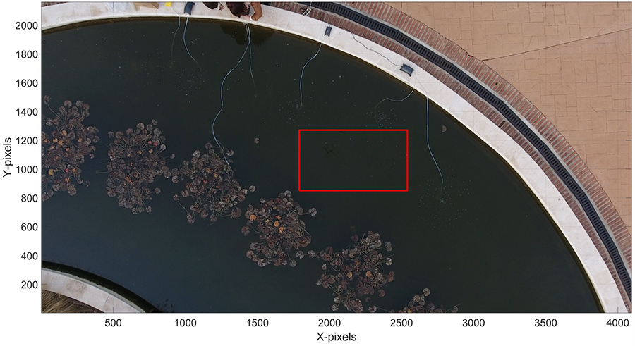
Figure 1. A single frame from the original footage with the region selected for the processing highlighted in red.

Figura 1. Fotograma de la grabación original, con la región seleccionada para el tratamiento resaltada en rojo.

The resulting image was converted to grayscale retaining its luminance, as the weighted average of the three channels:

(2)

The grayscale image was submitted to the Sobel-Feldman method to detect edges. The algorithm consists on finding the maximum and gradients of the image by convolving it with the following 3x3 matrixes (Sobel operator - Parker 2010):

(3)

The gradients and are the approximate derivative of the original image , where the symbol denotes the convolution. The magnitude of gradient is defined in each pixel of the image, as gray tones / pixel . Each pixel that exceeds the threshold of 0.1 is labeled as edge and associated to 1 in the output logical matrix.

Successively, contours smaller than 2x2 pixels, which may be bubbles with diameter of 4.7 mm or more often false detections, were discarded, and the number of pixels contained within the edge were counted for each isolated contour (a contour with at least one empty pixel (non-edge) distance from another). Therefore, the surface of each closed contour, has been calculated as:

(4)

where is the total number of pixels detected inside the contour plus the ones that shape the contour itself. Finally, the equivalent diameter of the bubble was defined as:

(5)

The whole sequence of processing steps described so far was iteratively applied to each frame of one of the test footages captured during the experiment. The whole process is very efficient: the area presented in this study is processed nearly in real time in a medium-high performance machine.

A real-time graphic interface was developed in MATLAB with the aim of assisting the user in the fine tuning of the processing parameters (Fig. 2).

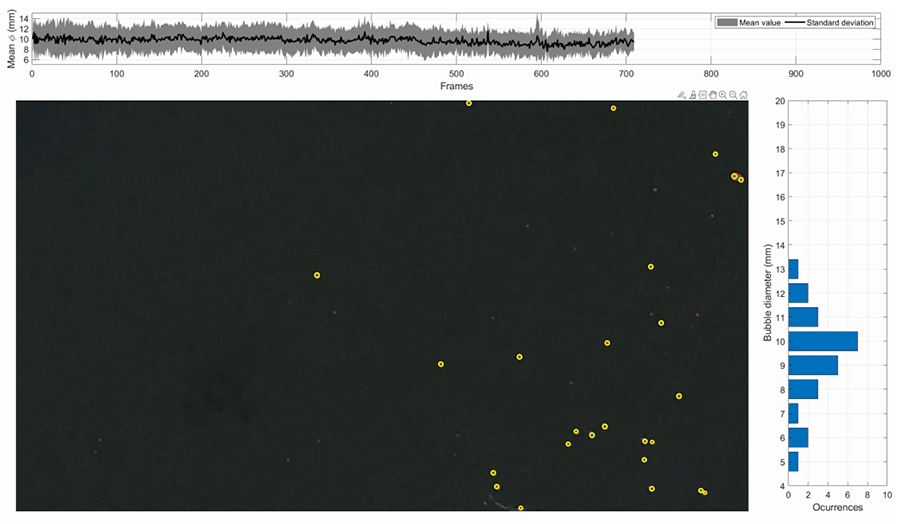
Figure 2. Interface developed in MATLAB to supervise the bubble detection algorithm (paused at frame 709). Top panel: time series of mean and standard deviation of bubbles diameter. Right panel: histogram of bubbles diameter for the current frame. Central panel: RGB frame, with detected contours in red line, and bubbles represented as yellow circle centered in the middle of each contour.

Figura 2. Interfaz desarrollada en MATLAB para supervisar el algoritmo de detección de burbujas (pausado en el fotograma 709). Panel superior: series temporales de media y desviación estándar de diámetro de burbujas. Panel derecho: histograma del diámetro de burbujas para el fotograma actual. Panel central: marco RGB, con el borde detectado en una línea roja y las burbujas representadas como un círculo amarillo centrado en el medio de cada contorno.

The current frame is displayed in real time in the central panel, and the detected bubbles are depicted as yellow circles located at the centroid of the pixels forming a contour, with the diameter calculated by equation (5). Above, the time series of the mean and standard deviation of the bubble’s diameter is built as the time goes forward. Finally, the right panel shows the histogram of bubbles diameter detected in the current frame.

On average, the interface reveals accurate detections of the bubbles, evaluated by visually comparing the size and position of the bubbles and the shape and extension of the red edges. Sporadically the bubbles agglomeration, typically provoked by the surface cohesion of few neighbor bubbles, are detected as one bigger bubble, or as few smaller ones, randomly located within the detected edge (see, for instance the two close bubbles detected at the upper right corner of main panel of Fig. 2). Notice that the performance of the detection algorithm is strictly related with the luminance contrast of the water surface and the bubbles. Any factor influencing this factor, as the generation of waves driven by wind, a brighter color, a higher transparency of the water, or a scarce environmental illumination, may reduce the efficiency of the method.

Figura 3a shows the histogram of the bubble’s diameter detected through the experiment described above. Mean and median values are 9.7 and 10.1 mm, respectively (edges smaller than 2x2 pixels are the 28% of detections, on average). The distribution is quite asymmetric with a large tail at the right, reflecting the higher occurrence of diameters at the smaller classes. Bubbles sizes match well with the ones visually inspected during the experiment and is coherent with the porosity of the air stone used by the air generators.

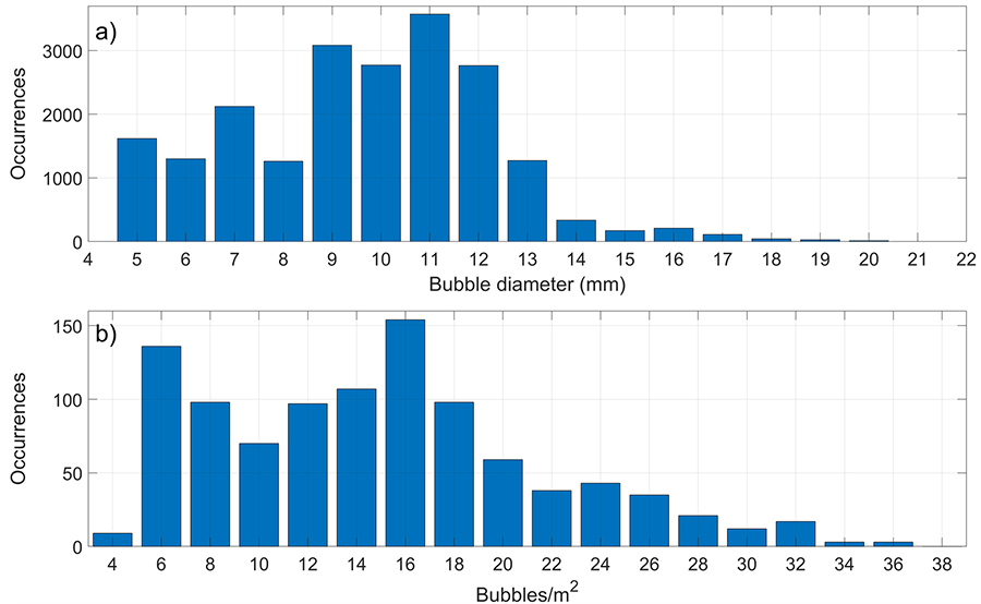
Figure 3. Panel a) Histogram of bubbles diameter calculated on the 1000 frames analyzed as a test experiment. Panel b) Histogram of bubbles per square meter detected throughout the whole experiment.

Figura 3. Panel a) Histograma de diámetro de burbujas calculado en los 1000 fotogramas analizados como experimento de prueba. Panel b) Histograma de burbujas por metro cuadrado detectadas a lo largo de todo el experimento.

Figura 3b shows the histogram of the number of bubbles detected per square meter (bubble density). The distribution may reflect the rate of air flow employed during the experiment, which was not necessarily constant. Two well differentiable maxima appear, centered around 6 bubbles/m²and 16 bubbles/m² respectively.

Our drone-based method offers valuable insights into methane bubble emissions in aquatic ecosystems, advancing the understanding of key features such as bubble size-abundance distributions and the spatial patterns of bubble plumes. This approach can complement traditional emission data, providing a more comprehensive view of methane dynamics in waterbodies, which is crucial for ecologists and biogeochemists studying greenhouse gas fluxes.

With an order of magnitude of few tens of square meters as the size of the total covered area used in this experiment, a full coverage of a whole basin turns up as rather infeasible. However, we can easily assume that a random distribution of a reduced number of small areas to be covered by single flights, throughout the whole region, may reasonably assure a good reproducibility of the average methane bubbling of the site. With this assumption, the scalability of the proposed method may be based on averaging the results of the whole series of flights.

The original MATLAB code of the algorithm presented in this study is available at https://github.com/simonesammartino/BubbleDetection, along with a short excerpt of the original footage to test the code.

Authors contribution

Sofía Rodríguez-Gómez: Methodology, investigation, writing-review and editing; Simone Sammartino: Methodology, formal analysis, investigation, software, writing-original draft; Miriam Ruiz-Nieto: Resources, methodology, investigation, writing-review and editing; Paula Warren-Jiménez: Methodology, writing-review and editing; Enrique Moreno-Ostos: Supervision, conceptualization, investigation, methodology, writing first draft, funding acquisition, project administration.

Acknowledgements

This study was funded by the Spanish Ministry of Science, Innovation and Universities through the Alter-C project (PID2020-114024GB-C33). Sofía Rodríguez-Gómez was funded by the Spanish Ministry of Science, Innovation and Universities through FPU22/01818 predoctoral contract.

References

Beaulieu, J.J., Smolenski, R.L., Nietch, C.T., Townsend-Small, A., Elovitz, M.S. 2014. High methane emissions from a midlatitude reservoir draining an agricultural watershed. Environmental Science and Technology 48(19), 11100-11108. https://doi.org/10.1021/es501871g

Deemer, B.R., Harrison, J.A., Li, S., Beaulieu, J.J., DelSontro, T., Barros, N., et al. 2016. Greenhouse gas emissions from reservoir water surfaces: A new global synthesis. BioScience 66(11), 949-964. https://doi.org/10.1093/biosci/biw117

Dooley, J.F., Minschwaner, K., Dubey, M.K., El Abbadi, S.H., Sherwin, E.D., Meyer, A.G., Follansbee, E., Lee, J.E. 2024. A new aerial approach for quantifying and attributing methane emissions: implementation and validation. Atmospheric Measurement Techniques 17, 5091-5111. https://doi.org/10.5194/amt-17-5091-2024

Green, D.R. 2020. Unmanned Aerial Remote Sensing: UAS for Environmental Applications. CRC Press. https://doi.org/10.1201/9780429172410

Hollenbeck, D., Zulevic, D., Chen, Y. 2021. Advanced Leak Detection and Quantification of Methane Emissions Using sUAS. Drones 5, 117. https://doi.org/10.3390/drones5040117

Lindgren, P., Grosse., G., Meyer, F.J., Anthon., K.W. 2019. An Object-Based Classification Method to Detect Methane Ebullition Bubbles in Early Winter Lake Ice. Remote Sensing 11, 822. https://doi.org/10.3390/rs11070822

Matthews, E., Johnson, M.S., Genovese, V., Du, J., Bastviken, D. 2020. Methane emission from high latitude lakes: methane‑centric lake classification and satellite‑driven annual cycle of emissions. Scientific Reports 10, 12465. https://doi.org/10.1038/s41598-020-68246-1

McNicol, G., Fluet-Chouinard, E., Ouyang, Z., Knox, S., Zhang, Z., Aalto. T., et al. 2023. Upscaling Wetland Methane Emissions From the FLUXNET-CH4 Eddy Covariance Network (UpCH4 v1.0): Model Development, Network Assessment, and Budget Comparison. AGU Advances 4: e2023AV000956. https://doi.org/10.1029/2023AV000956

Montes-Pérez, J.J., Obrador, B., Conejo-Orosa, T., Rodríguez, V., Marcé, R., Escot, C., Reyes, I., et al. 2022. Spatio-temporal variability of carbon dioxide and methane emissions from a Mediterranean reservoir. Limnetica 41(1), 43-60. https://doi.org/10.23818/limn.41.04

Myhre, G., Shindell, D., Bréon, F.M., Collins, JW., Fuglestvedt, J., Huang, J., Koch, D., et al. 2013. Anthropogenic and natural radiative forcing. In: Stocker, T.F., Qin, D., Plattner, G.-K., Tingor, M., Allen, S.k., Doschung, J., Nauels, A., et al. (Eds.). Climate Change 2013: The physical science basis. Contribution of working group I to the Fifth Assessment Report of the Intergovernmental Panel on Climate Change. Cambridge University Press, Cambridge, United Kingdom and New York, USA. https://doi.org/10.1017/CBO9781107415324.018

Ostrovsky, I., McGinnins, D.F., Lapidus, L., Eckert, W. 2008. Quantifying gas ebullition with echosounder: the role of methane transport by bubbles in a medium-sized lake. Limnology and Oceanography: Methods 6: 105-118. https://doi.org/10.4319/lom.2008.6.105

Parker, J.R. 2010. Algorithms for Image Processing and Computer Vision. John Wiley & Sons.

Vélez, A.F., Álvarez, C.I., Navarro, F., Guzmán, D., Bohórquez, M.P., Gómez Selvaraj, M., Ishitani, M. 2024. Assessing methane emissions from paddy fields through environmental and UAV remote sensing variables. Environmental Monitoring and Assessment 196: 574. https://doi.org/10.1007/s10661-024-12725-9

Villa, J.A., Ju, Y.,Yazbeck, T., Waldo, S.,Wrighton, K.C., Bohrer, G. 2021. Ebullition dominates methane fluxes from the water surface across different ecohydrological patches in a temperate freshwater marsh at the end of the growing season. Science of the Total Environment 767: 144498. https://doi.org/10.1016/j.scitotenv.2020.144498

Walter, K.M., Engram, M., Duguay, C.R., Jeffries, M.O., Chapin, F.S. 2008. The potential use of synthetic aperture radar for estimating methane ebullition from Arctic lakes. Journal of the American Water Resources Association 44(2): 305-315. https://doi.org/10.1111/j.1752-1688.2007.00163.x